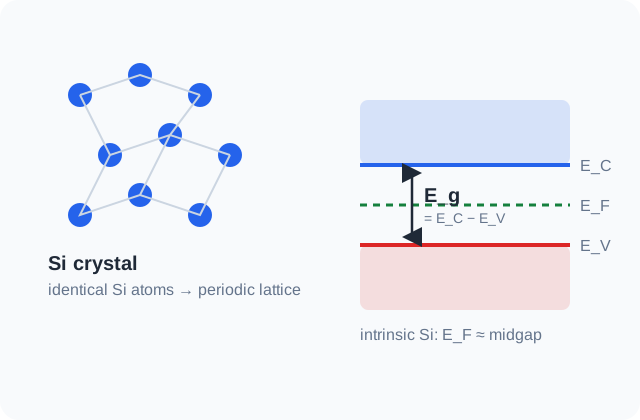
1. AtomSi atomunun dört değerlik elektronu vardır.
2. KristalKomşu Si atomları kovalent bağlarla periyodik örgü kurar.
3. Enerji bantlarıAtomik seviyeler valans ve iletim bantlarına dönüşür.
4. TaşıyıcıUyarılan elektron hareket eder; geride hareketli bir hol kalır.
Kristal örgü ve enerji bantlarının ilişkisi · Özgün teknik şema
1.1 Kristal yapı
Neden kristal yapı ile başlıyoruz? Kristal yapı zorunlu mu?
Hayır; bir malzemenin yarıiletken olması için mutlaka kristal olması gerekmez. Yarıiletken olmayı belirleyen şey “kristal olması” değil, elektronik durumlarının valans ve iletim bölgeleri oluşturması ve elektriksel iletkenliğinin sıcaklık, katkılama, ışık veya elektrik alan gibi etkilerle kontrol edilebilir olmasıdır. Kristal yapı bunu özellikle temiz ve hesaplanabilir hale getirir: atomların periyodik dizilimi sayesinde (E(\mathbf{k})) bant yapısı, kristal momentumu, etkin kütle ve taşıyıcı hareketliliği gibi kavramlar iyi tanımlanır.
Bu nedenle yüksek performanslı klasik aygıtların aktif bölgeleri çoğunlukla tek kristal veya epitaksiyel kristal Si, GaAs, GaN ya da SiC'den yapılır. Ancak polikristal Si (ör. bazı TFT ve güneş hücreleri), amorf Si:H ve amorf oksit yarıiletkenler (ör. IGZO) da gerçek yarıiletkenlerdir. Kristal olmayan malzemelerde uzun menzilli periyodiklik kaybolduğu için ders boyunca sık kullanacağımız düzgün (E(\mathbf{k})) resmi daha sınırlı hale gelir; bu yüzden temel fiziğe kristal yarıiletkenlerle başlamak en temiz başlangıçtır.
Si, Ge ve GaAs gibi yarı iletkenler düzenli bir kristal örgüde bulunur. Si ve Ge elmas yapısında, GaAs ise çinko sülfür (zincblende) yapısında kristalleşir. Her iki yapı da birbirinin içine geçmiş iki yüzey merkezli kübik (fcc) alt örgüden oluşur; ikinci alt örgü, birinciye göre cisim köşegeni boyunca \(a/4\) kaydırılmıştır. Böylece her atom dört en yakın komşusuyla düzgün dört yüzlü (tetrahedral) kovalent bağlar kurar. Elmas yapıda iki alt örgünün atomları aynı türdendir, zincblende'de ise bir alt örgü Ga, diğeri As'tır.
Oda sıcaklığında Si'nin örgü sabiti \(a = 5.431\) Å, GaAs'ınki \(a = 5.653\) Å'dur. Kristal düzlemleri ve yönleri Miller indisleriyle \((hkl)\) ve \([hkl]\) olarak gösterilir; entegre devre üretiminde çoğunlukla (100) yüzeyli pullar kullanılır, çünkü bu yüzeyde oksit–yarı iletken ara yüzey tuzak yoğunluğu en düşüktür.
1.2 Enerji bantları
Atomlar kristal oluşturmak üzere yaklaştıkça, tek atomdaki keskin enerji seviyeleri Pauli ilkesi gereği yarılarak bantlara dönüşür. Yarı iletkende 0 K'de tamamen dolu en üst banda valans bandı, tamamen boş en alt banda iletim bandı denir; ikisi arasındaki yasak aralık bant aralığı \(E_g\)'dir. Si için oda sıcaklığında \(E_g = 1.12\) eV, GaAs için 1.42 eV, Ge için 0.66 eV'dur.
Bu değerler büyük mü, küçük mü? 1 eV ile kıyaslama
1 eV, bir elektronun 1 V'luk potansiyel farkını geçerken kazandığı enerjidir: \(1\ \mathrm{eV}=1.602\times10^{-19}\) J. Tek bir elektron için anlamlı bir enerji, gündelik ölçekte ise çok küçüktür: 1 J yaklaşık \(6\times10^{18}\) eV eder. Si'nin 1.12 eV'luk bant aralığının “büyük” mü “küçük” mü olduğunu, onu aynı ölçekteki başka enerjilerle karşılaştırarak anlarız:
Enerji ölçeği
Değer
Si'nin \(E_g\)'siyle (1.12 eV) kıyas
Oda sıcaklığında ısıl enerji \(kT\) (300 K)
0.026 eV
\(E_g\approx43\,kT\): ısı tek başına bağları çok nadir koparır; bu yüzden \(n_i\) küçüktür.
Si'de P donörünün iyonlaşma enerjisi
0.045 eV
\(\approx E_g/25\): donörler oda sıcaklığında kolayca iyonlaşır.
Si'deki en enerjik (optik) fonon
0.063 eV
\(\approx E_g/18\): tek bir fonon elektronu valans bandından iletim bandına taşıyamaz.
1 eV'luk foton
\(\lambda\approx1240\) nm (yakın kızılötesi)
Si'nin bant aralığına çok yakın. Genel kural \(\lambda_c=1240/E_g\) → Si ≈ 1110 nm'den uzun dalgaları soğuramaz.
Görünür ışık fotonu
1.65–3.3 eV (750–380 nm)
\(E_g\)'den büyük: Si görünür ışığın tamamını soğurur, bu yüzden koyu gri görünür ve güneş hücresi yapılabilir.
Si–Si kovalent bağ enerjisi
≈ 2.3 eV
Bir elektronu iletim bandına çıkarmak, bağı tamamen koparmaktan ucuzdur; kristal dağılmaz.
Hidrojen atomunu iyonlaştırma
13.6 eV
≈ 12 × \(E_g\): kristalde bir elektronu hareketli hale getirmek, serbest bir atomdan koparmaktan çok daha kolaydır.
Tıbbi X-ışını fotonu
20–150 keV
On binlerce kat büyük: tek foton çok sayıda elektron–hol çifti üretir (X-ışını dedektörlerinin ilkesi).
Elektronun durgun kütle enerjisi \(m_0c^2\)
511 keV
≈ 450 000 × \(E_g\): yarıiletken olayları göreli (relativistik) değildir.
Sıcaklık karşılığı \(E/k\)
1 eV ≈ 11 600 K
Si'nin \(E_g\)'si ≈ 13 000 K'e karşılık gelir. Aygıtlar bundan çok düşük sıcaklıkta çalıştığı için taşıyıcılar dağılımın üstel kuyruğundan gelir.
Başka malzemelerle kıyas. Bant aralığı malzemeden malzemeye yüzlerce kat değişir ve katının karakterini belirler:
Sınıf
Örnekler (300 K, \(E_g\) eV)
Sonuç
Metal
Cu, Al: 0 (bantlar örtüşür)
Her sıcaklıkta çok sayıda serbest elektron; iletkenlik sıcaklıkla hafifçe düşer.
Dar aralıklı yarıiletken
InSb 0.17 · InAs 0.35 · PbS 0.41
Kızılötesi dedektörler. Oda sıcaklığında \(n_i\) büyüktür; çoğu zaman soğutma gerekir.
“Klasik” yarıiletken
Ge 0.66 · Si 1.12 · InP 1.34 · GaAs 1.42 · CdTe 1.5
Elektronik ve güneş hücreleri: \(E_g\approx1\) eV civarı, katkıyla kontrol edilebilen taşıyıcı sayısı.
Geniş aralıklı yarıiletken
GaP 2.26 · 4H-SiC 3.26 · ZnO 3.37 · GaN 3.4
Yüksek gerilim ve sıcaklıkta çalışan güç aygıtları, mavi–UV LED'ler.
Ultra geniş aralık / yalıtkan
Elmas 5.5 · AlN 6.1 · SiO₂ ≈ 9
Neredeyse hiç ısıl taşıyıcı yoktur; SiO₂ MOSFET'in kapı yalıtkanıdır.
Kaba kural olarak belirleyici olan \(E_g/kT\) oranıdır: oda sıcaklığında InSb için ≈ 7 (taşıyıcı bol), Si için ≈ 43 ve GaAs için ≈ 55 (katkıyla kontrol edilebilir), GaN için ≈ 130 ve SiO₂ için ≈ 350 (taşıyıcı yok denecek kadar az). Si, 1 eV'a çok yakın bant aralığıyla bu ölçeğin tam ortasındadır. Görseller sekmesindeki bant aralığı ölçeği grafiğinde bu malzemeleri farklı sıcaklıklarda karşılaştırabilirsiniz.
Bant yapısı, enerjinin kristal momentumuna \(\hbar\mathbf{k}\) bağlılığı \(E(\mathbf{k})\) ile tanımlanır. İletim bandı minimumu ile valans bandı maksimumu aynı \(\mathbf{k}\) değerindeyse yarı iletken doğrudan bant aralıklıdır (GaAs). Farklı \(\mathbf{k}\) değerlerindeyse dolaylı bant aralıklıdır (Si, Ge). Dolaylı geçişlerde momentum korunumu için bir fononun katılması gerekir; bu yüzden Si verimli ışık yayamaz, GaAs ise LED ve lazerlerde kullanılır. Bu ayrımı Görseller sekmesindeki 3B \(E(k)\) yüzeyinde inceleyebilirsiniz.
Bant kenarlarının yakınında \(E(k)\) parabol ile yaklaşılabilir ve eğrilik etkin kütle \(m^*\) ile ifade edilir. Etkin kütle, kristalin periyodik potansiyelinin etkisini taşıyıcının kütlesine gömer; böylece elektron ve hollere dış kuvvetler altında serbest parçacık gibi davranan nesneler olarak bakabiliriz.
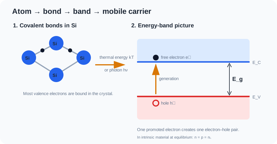
Kovalent bağdan kopan bir elektron, bant resminde iletim bandına çıkar ve aynı olayda bir hol oluşur · Özgün teknik şema
1.3 Serbest elektron ve hol
Serbest elektron nedir?
Kristaldeki bütün elektronlar akıma eşit katkı vermez. Si değerlik elektronlarının çoğu kovalent bağların parçasıdır ve bağlı durumdadır. Bir elektron ısı veya ışıkla yeterli enerji kazanıp valans bandından iletim bandına geçtiğinde, bant içindeki boş durumlara geçebilir ve elektrik alan altında sürüklenebilir. Bu elektron artık serbest elektron taşıyıcısıdır.
Buradaki “serbest”, vakumdaki serbest elektron anlamına gelmez. Elektron hâlâ kristalin periyodik potansiyelini hisseder; bu etki etkin kütle \(m^*\) gibi büyüklüklerle modele katılır.
Hol (boşluk) nedir?
Bir elektron valans bandından ayrıldığında arkasında dolmamış bir durum bırakır. Komşu bir elektron bu boşluğu doldurunca boşluk başka yere geçmiş gibi görünür. Bu kolektif hareketi hol olarak modelleriz ve hol pozitif yük \(+q\) taşıyan bir yarı-parçacık gibi davranır.
Önemli: Hol yeni bir temel parçacık değildir; valans bandındaki elektron eksikliğinin kullanışlı fiziksel modelidir.
Akımı ne oluşturur?
Elektrik akımı, yükün belirli bir yönde net hareketidir: \(J = q\,(p\,\bar v_p - n\,\bar v_n)\). Buradan iki koşul çıkar: ortamda hareket edebilen yük taşıyıcıları olmalı ve bu taşıyıcıların hareketi bir yöne ortalama olarak kaymalıdır. Oda sıcaklığında taşıyıcılar zaten ~\(10^7\) cm/s ısıl hızla koşar, ama yönleri rastgele olduğu için ortalamaları sıfırdır ve akım oluşmaz.
Bağlı elektronlar neden akım taşımaz? Tamamen dolu bir bantta her \(\mathbf{k}\) durumundaki elektronun karşısında \(-\mathbf{k}\) durumunda da bir elektron vardır; toplam momentum sıfırdır. Alan elektronları itmek istese de geçebilecekleri boş durum yoktur, bu yüzden dağılım değişmez ve net akım sıfır kalır. Tamamen boş bantta ise zaten taşıyıcı yoktur. Akımı yalnızca kısmen dolu bantlar taşır: iletim bandındaki az sayıdaki elektron ve valans bandındaki az sayıdaki boş durum (hol). Valans bandının geri kalan milyarlarca elektronu akıma ancak holler üzerinden katkı verir.
Katkılama: iyonlaşan donör/akseptörler → \(n\approx N_D\) veya \(p\approx N_A\) (1.5–1.7).
Optik üretim: \(h\nu\ge E_g\) fotonların soğurulması → güneş hücresi, fotodiyot.
Enjeksiyon: kontaktan veya p-n ekleminden taşıyıcı girmesi → diyot ve BJT (2.–3. ve 9. hafta).
Çığ ve tünelleme: çok yüksek alanda çarpışmalı iyonlaşma veya bant-bant tünelleme → kırılma, tünel diyot (3.–4. hafta).
2. Onları ne hareket ettirir? (“hangi yöne?”)
Sürüklenme (drift): elektrik alan. Elektronlar alana ters, holler alan yönünde gider, ama iki akım aynı yönde toplanır: \(J=q(n\mu_n+p\mu_p)\mathcal{E}\).
Difüzyon: yoğunluk farkı; taşıyıcılar çoktan aza yayılır (1.12). p-n ekleminin ve BJT tabanının ana akımı budur.
Sıcaklık farkı: sıcak uçtaki taşıyıcılar daha hızlıdır → termoelektrik (Seebeck) akımı; termoelektrik soğutucu ve jeneratörler.
Yer değiştirme akımı: \(\varepsilon\,\partial\mathcal{E}/\partial t\); yük karşıya geçmeden, değişen alanla akan kapasitif akım. Yüksek frekansta önemlidir (11. hafta).
Kısacası akım, taşıyıcı sayısı (\(n,p\)) ile hareket kolaylığının (\(\mu\)) çarpımı ve bir itici etken (alan, yoğunluk veya sıcaklık farkı) ile belirlenir: \(\sigma=q(n\mu_n+p\mu_p)\). Bunun sayısal etkisi çok büyüktür. Saf Si'de 300 K'de \(\rho\approx3\times10^{5}\ \Omega\,\mathrm{cm}\) iken \(N_D=10^{16}\ \mathrm{cm^{-3}}\) katkılı Si'de \(\rho\approx0.5\ \Omega\,\mathrm{cm}\) olur. Karşılaştırma için bakırda \(\rho\approx1.7\times10^{-6}\ \Omega\,\mathrm{cm}\)'dir.
1.4 Isıl dengede taşıyıcılar ve \(n_i\)
Bir enerji seviyesinin elektronla dolu olma olasılığı Fermi–Dirac dağılımıyla verilir. Fermi seviyesi \(E_F\), doluluk olasılığının tam 1/2 olduğu enerjidir. İletim bandındaki elektron yoğunluğu, durum yoğunluğu ile doluluk olasılığının çarpımının bant boyunca integralidir. \(E_F\), bant kenarlarından birkaç \(kT\) uzakta olduğu sürece (dejenere olmayan durum) bu integral basit bir üstel ifadeye indirgenir.
Intrinsic carrier concentration veya öz taşıyıcı yoğunluğu \(n_i\), katkısız bir yarıiletkende termal dengede birim hacimde doğal olarak bulunan hareketli elektron ve hol yoğunluğudur. Intrinsic malzemede her kopan bağ bir elektron ve bir hol ürettiği için:
\[\boxed{n=p=n_i}\]
Si için 300 K'de \(n_i\approx9.65\times10^{9}\ \mathrm{cm^{-3}}\) (Sze 3. baskı; eski kaynaklarda \(1.45\times10^{10}\) değeri geçer). Bu değer Si atom yoğunluğu değildir: 1 cm³ silisyumda yaklaşık \(5\times10^{22}\) atom vardır; yani saf Si'de oda sıcaklığında her ~\(5\times10^{12}\) atoma yalnızca bir serbest elektron düşer. Saf silisyum bu yüzden iyi bir iletken değildir.
\(N_C\) ve \(N_V\) yaklaşık \(T^{3/2}\) ile değişse de baskın etki üstel terimdir. Sıcaklık arttıkça daha fazla elektron bant aralığını aşar ve \(n_i\) hızla büyür: Si'de 300 K'den 400 K'e çıkınca \(n_i\) yaklaşık 500 kat artar. \(E_g\) büyüdükçe aynı sıcaklıkta intrinsic taşıyıcı üretimi azalır.
Bu üstel bağımlılık, yarıiletken aygıtların sıcaklığa duyarlılığının temel nedenidir.
Isıl denge pratikte ne demek? Kararlı durum (steady state) ile farkı
Isıl denge, malzemeye dışarıdan hiç enerji verilmediği ve her yerin aynı sıcaklıkta olduğu, yeterince uzun süre beklenmiş durumdur: uygulanan gerilim yok, ışık yok, sıcaklık farkı yok. Bu durumda her mikroskobik süreç kendi tersiyle dengelenir (ayrıntılı denge):
Isıl üretim hızı rekombinasyon hızına eşittir: \(G=R\). Taşıyıcılar sürekli oluşup yok olur, ama sayıları sabit kalır.
Elektron akımı ve hol akımı ayrı ayrı sıfırdır; bir yerde sürüklenme varsa onu tam dengeleyen bir difüzyon vardır (p-n ekleminde olduğu gibi).
Fermi seviyesi \(E_F\) her yerde sabittir ve \(np=n_i^2\) geçerlidir.
Denge durgunluk değildir: taşıyıcılar ısıl hızla koşmaya, üretilip yok olmaya devam eder. Yalnızca her şeyin net sonucu sıfırdır.
Kararlı durum (steady state) ise büyüklüklerin zamanla değişmediği (\(\partial/\partial t=0\)) ama sistemin sürekli enerji aldığı ve bir şeyin aktığı durumdur. Sabit bir gerilim veya sabit bir ışık, taşıyıcıları sürekli üretir ya da enjekte eder; aynı hızla rekombinasyon ve akım onları götürür. Değerler sabittir ama akım sıfır değildir, \(G\ne R_{\text{ısıl}}\) olabilir ve \(np\ne n_i^2\) olur. Her ısıl denge bir kararlı durumdur; tersi doğru değildir. Zamanla değişen durumlara ise geçici durum (transient) denir.
Pratik durum
Hangisi?
Neden
Rafta duran, bağlı olmayan çip (karanlık, oda sıcaklığı)
Isıl denge
Dışarıdan enerji yok; tüm akımlar sıfır.
Açık devre p-n eklemi, karanlıkta
Isıl denge
Eklemde yerleşik gerilim \(V_{bi}\) ve alan vardır ama sürüklenme ile difüzyon birbirini tam dengeler; akım sıfırdır (2. hafta).
Sabit DC gerilimde çalışan diyot veya transistör
Kararlı durum
Akım sabit ama sıfır değil; eklem çevresinde \(np\ne n_i^2\).
Sabit ışık altındaki güneş hücresi veya fotodiyot
Kararlı durum
Optik üretim sürekli; fazla taşıyıcı yoğunluğu sabit ama dengedekinden fazla.
Anahtarlanan transistör, ışık darbesi (Haynes–Shockley), açılış anı
Geçici durum
Yoğunluklar ve akımlar zamanla değişir (13. hafta).
Gerilim veya ışık kesildikten hemen sonra
Geçici → denge
Fazla taşıyıcılar ömür \(\tau\) (Si'de ns–ms) içinde rekombine olur ve sistem dengeye döner.
Denge formülleri neden hâlâ işe yarar? Aygıt çalışırken bile her bant içindeki taşıyıcılar fononlarla çok hızlı (~ps) ısınıp soğur ve kendi içinde dengeye gelir. Bu yüzden kararlı durumda her bant için ayrı bir yarı-Fermi seviyesi tanımlanabilir ve denge denklemleri küçük düzeltmelerle kullanılır. Ayrıca düşük enjeksiyonda çoğunluk taşıyıcı yoğunluğu dengedeki değerine çok yakındır; derste “ısıl dengedeki” değerler, aygıt analizinin başlangıç noktasıdır.
1.5 Katkılama: taşıyıcı sayısını neden ve nasıl seçeriz?
Saf silisyumun iki sorunu vardır: taşıyıcı sayısı çok azdır ve bu sayı sıcaklıkla üstel olarak değişir. Çözüm, kristale kontrollü miktarda yabancı atom (katkı, dopant) yerleştirmektir. Katkı atomu bir Si atomunun yerine oturur (yer değiştirmeli katkı) ve dört komşusuyla bağ kurar. Katkının değerlik elektron sayısı Si'den farklı olduğu için bir elektron artar ya da eksik kalır; taşıyıcı sayısını artık sıcaklık değil, üretim sırasında seçtiğimiz katkı miktarı belirler.
1.6 \(N_D\) ve \(N_A\): katkı yoğunluğu tanımı
Katkı miktarını, birim hacimdeki katkı atomu sayısıyla ölçeriz. Bu iki sembol dersin geri kalanında her denklemde karşımıza çıkacak:
\(N_D\)donör (verici) yoğunluğu
Ne sayar?
Birim hacimdeki donör atomu sayısı: V. grup atomları (P, As, Sb). Her biri kristale bir fazla elektron “verir”.
Birim
\(\mathrm{cm^{-3}}\) (atom / cm³)
İyonlaşmış kısmı
\(N_D^+\): elektronunu iletim bandına bırakmış, geride sabit \(+q\) yük kalan donörler. Oda sıcaklığında Si'de \(N_D^+\approx N_D\).
Sonucu
\(N_D\gg n_i\) ise \(n\approx N_D\) → n tipi
\(N_A\)akseptör (alıcı) yoğunluğu
Ne sayar?
Birim hacimdeki akseptör atomu sayısı: III. grup atomları (B, Al, Ga). Her biri valans bandından bir elektron “alır”.
Birim
\(\mathrm{cm^{-3}}\) (atom / cm³)
İyonlaşmış kısmı
\(N_A^-\): valans bandından elektron yakalamış, geride sabit \(-q\) yük ve hareketli bir hol bırakan akseptörler.
Sonucu
\(N_A\gg n_i\) ise \(p\approx N_A\) → p tipi
\(N_D\) ile \(n\) aynı şey değildir: \(N_D\) kaç tane katkı atomu koyduğumuzu, \(n\) ise kaç tane elektronun gerçekten hareket edebildiğini sayar. İkisinin eşit olması (\(n\approx N_D\)) ancak donörlerin hepsi iyonlaştığında ve \(N_D\gg n_i\) olduğunda geçerli bir yaklaşımdır. Katkının ne kadar “seyreltik” olduğunu görmek için Si atom yoğunluğuyla karşılaştıralım:
\(N_D\) veya \(N_A\) (cm⁻³)
Kaç Si atomuna 1 katkı?
Tipik kullanım
\(10^{14}\)
~ 500 milyon
çok hafif katkı; güç aygıtı sürüklenme bölgesi, dedektör
\(10^{15}\)–\(10^{16}\)
~ 50 milyon – 5 milyon
hafif katkı; pul (wafer) tabanı, BJT kolektörü
\(10^{17}\)–\(10^{18}\)
~ 500 bin – 50 bin
orta/yüksek katkı; BJT tabanı, MOSFET kanal ayarı
\(\gtrsim 10^{19}\)
~ 5 bin veya daha az
yoğun katkı (\(n^+\), \(p^+\)); kontaklar, emetör, kaynak/savak
Kompanzasyon: Aynı bölgede hem donör hem akseptör varsa ikisi birbirini kısmen yok eder; donörün fazla elektronu akseptörün eksiğini doldurur. Tip ve çoğunluk taşıyıcı yoğunluğu net katkıyla belirlenir: \(N_D>N_A\) ise \(n\approx N_D-N_A\), \(N_A>N_D\) ise \(p\approx N_A-N_D\).
1.7 n tipi ve p tipi silisyum
n tipi silisyum (negatif taşıyıcı çoğunlukta)
Nasıl yapılır? Si'ye V. grup atomu (P, As, Sb) eklenir: \(N_D>N_A\).
Mikroskobik resim: P'nin 5 değerlik elektronundan 4'ü komşu Si'lerle bağ kurar; 5. elektron çok zayıf bağlıdır.
Bant resmi: Donör seviyesi \(E_D\), \(E_C\)'nin yalnızca ~45 meV altındadır (\(kT\approx26\) meV). Oda sıcaklığında neredeyse tüm donörler iyonlaşır.
Geride kalan: hareket edemeyen \(\mathrm{P^+}\) iyonu. Hol oluşmaz.
İki tip de aynı kristaldir; farkı milyonlarca atomda bir yer alan katkı atomları yaratır. Buna rağmen etkisi çok büyüktür: \(N_D=10^{16}\ \mathrm{cm^{-3}}\) ile elektron yoğunluğu \(n_i\)'nin yaklaşık bir milyon katına çıkar, hol yoğunluğu ise yaklaşık bir milyon kat azalır. p-n eklemi, BJT ve MOSFET gibi aygıtların hepsi n ve p bölgelerinin yan yana getirilmesiyle çalışır.
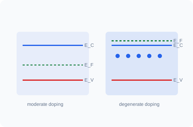
Katkı arttıkça \(E_F\) ilgili bant kenarına yaklaşır. \(N_D\) yaklaşık \(10^{18}\ \text{cm}^{-3}\)'ün üzerine çıktığında Boltzmann yaklaşımı bozulmaya başlar; bu durum 5. haftada yüksek katkılama etkileri başlığında ele alınacaktır.
1.8 Kütle etkisi yasası: katkılama varken \(n_i\)
Katkılama \(n_i\)'yi ortadan kaldırmaz. Donör veya akseptörler çoğunluk taşıyıcısını değiştirir; termal dengede ise çarpım sabit kalır (kütle etkisi yasası):
\[\boxed{np=n_i^2}\]
Çoğunluk taşıyıcısı artarsa, fazla elektronlar holler ile daha sık karşılaşıp rekombine olduğu için azınlık taşıyıcısı aynı oranda azalır. Tam iyonlaşmış, kompanzasyonsuz n tipi malzemede \(N_D\gg n_i\) ise \(n\approx N_D\) ve \(p\approx n_i^2/N_D\) olur.
Üç yoğunluğu karıştırmayın:Atom yoğunluğu kristaldeki atomları (\(\approx5\times10^{22}\ \mathrm{cm^{-3}}\)), katkı yoğunluğu (\(N_D\), \(N_A\)) eklenen donör/akseptörleri, taşıyıcı yoğunluğu (\(n\), \(p\), \(n_i\)) ise gerçekten hareket edebilen elektron ve holleri sayar. Görseller sekmesindeki çubuk grafikte üçünü aynı eksende karşılaştırabilirsiniz.
1.9 Dört oyuncu: elektron, hol, foton ve fonon
Yarıiletken fiziğinde olan biten neredeyse her şey dört “parçacık” arasındaki alışverişle anlatılır. Elektron ve hol yük taşır; foton ve fonon enerji ve momentum taşır, taşıyıcıları üretir, yok eder veya saptırır.
Oyuncu
Nedir?
Yük
Tipik enerji / momentum
Bu dersteki rolü
Elektron (e⁻)
İletim bandındaki hareketli elektron
\(-q\)
\(E\approx E_C+\tfrac32kT\)
akım taşır; n tipinde çoğunluk
Hol (h⁺)
Valans bandındaki elektron eksikliği (yarı-parçacık)
\(+q\)
\(E\approx E_V-\tfrac32kT\)
akım taşır; p tipinde çoğunluk
Foton (\(h\nu\))
Işık kuantumu
0
enerjisi büyük (~1 eV), momentumu çok küçük
soğurulunca e⁻–h⁺ çifti üretir; doğrudan rekombinasyonda salınır (LED, lazer)
Fonon
Örgü titreşiminin kuantumu (“ses/ısı paketi”)
0
enerjisi küçük (Si'de ≤ 63 meV), momentumu büyük olabilir
Bu dört oyuncunun karşılaştığı üç tipik sahne vardır:
Üretim: bir foton (\(h\nu\ge E_g\)) veya yeterince enerjik bir fonon bir bağı koparır → bir elektron + bir hol. Si dolaylı bant aralıklı olduğundan, bant kenarında foton soğurmasına momentum sağlamak için bir fonon da katılmalıdır.
Saçılma: hareket eden elektron ya da hol bir fononla veya iyonlaşmış katkı atomuyla etkileşip yön/hız değiştirir. Taşıyıcı yok olmaz, yalnızca rotası değişir. 1.10–1.12 bu olayı ele alır.
Rekombinasyon: elektron bir hol ile birleşir, çift yok olur. Enerji GaAs gibi doğrudan malzemede çoğunlukla foton (ışık), Si'de çoğunlukla tuzaklar üzerinden fonon (ısı) olarak açığa çıkar.
1.10 Çarpışma ve saçılma nedir? Farkı ne?
Çarpışmagünlük dildeki imge
Resim
İki bilardo topu gibi, birbirine değen iki cisim.
Katıda
Taşıyıcının hareketini kesen olay için kullanılan kısa ve sezgisel ad. Drude modelinde “ortalama çarpışma süresi” \(\tau\) diye anılır.
Sınırı
Taşıyıcının Si atomlarına fiziksel olarak toslaması değildir; o resim yanlış sayılar verir.
Saçılmafiziğin kullandığı kavram
Tanım
Taşıyıcının kristal momentumunun (ve bazen enerjisinin) kristalin mükemmel periyodikliğini bozan bir etki yüzünden aniden değişmesi.
Temas?
Gerekmez. İyonlaşmış bir katkının Coulomb alanı taşıyıcıyı uzaktan saptırır; bir fonon soğurulup salınabilir.
Türleri
Elastik (enerji neredeyse korunur, yalnız yön değişir) veya inelastik (fonon alışverişiyle enerji de değişir).
Kısacası: “çarpışma” olayın gündelik adı, “saçılma” fiziksel mekanizmasıdır. Bu derste ikisi aynı olayı anlatmak için kullanılabilir, ama sayılarla konuşurken saçılma resmini düşünmek gerekir. En şaşırtıcı nokta şudur: mükemmel ve titreşmeyen bir kristalde elektron hiç saçılmaz. Elektron bir dalgadır ve periyodik potansiyel içinde (Bloch dalgası olarak) engelsiz ilerler; atomların “etkisi” zaten etkin kütle \(m^*\)'ın içindedir. Direnci doğuran, bu periyodikliği bozan her şeydir.
Not: “Elektronlar Si atomlarına çarptığı için direnç oluşur.” Yanlış. Öyle olsaydı serbest yol atomlar arası mesafe (~0.2 nm) mertebesinde olurdu; ölçülen değer ise oda sıcaklığında onlarca nanometredir ve soğudukça uzar. Taşıyıcıyı saptıran atomların kendisi değil, titreşimleri (fononlar) ve kusurlardır.
1.11 Çarpışmalar nelerden oluyor?
1. Örgü (fonon) saçılması
Sıcaklıkta atomlar denge konumları etrafında titreşir; periyodiklik anlık olarak bozulur.
Akustik fononlar: düşük enerjili, yaklaşık elastik saçılma. Oda sıcaklığında hafif katkılı Si'de baskın mekanizma.
Optik fononlar: Si'de ~63 meV. Yüksek alanda hızlanan taşıyıcı enerjisini bunlara verir → sürüklenme hızı ~\(10^7\) cm/s'de doyar.
T arttıkça fonon sayısı artar: \(\mu_L\propto T^{-3/2}\).
2. İyonlaşmış katkı (Coulomb) saçılması
\(\mathrm{P^+}\) ve \(\mathrm{B^-}\) iyonları çevrelerinde Coulomb alanı yaratır ve taşıyıcıyı saptırır (Rutherford saçılmasına benzer).
Yavaş taşıyıcı daha çok sapar; yüksek sıcaklıkta taşıyıcılar hızlı olduğundan bu saçılma zayıflar.
Katkı arttıkça güçlenir: \(\mu_I\propto T^{3/2}/N_I\), \(N_I=N_D^++N_A^-\).
Düşük sıcaklıkta ve yoğun katkılı bölgelerde baskındır.
Diğer kaynaklar: nötr katkı atomları ve kristal kusurları (boşluk, dislokasyon), MOSFET kanalında oksit arayüzünün pürüzlülüğü, çok yüksek taşıyıcı yoğunluğunda taşıyıcı–taşıyıcı (elektron–elektron, elektron–hol) saçılması ve alaşımlarda (SiGe) alaşım düzensizliği. Holler de aynı mekanizmalarla saçılır; Si'de hol hareketliliğinin (\(\approx470\)) elektronunkinden (\(\approx1400\ \mathrm{cm^2/V\,s}\)) düşük olmasının ana nedeni holün daha büyük etkin kütlesidir.
1.12 Sürüklenme, hareketlilik ve difüzyon
Taşıyıcı iki saçılma arasında ısıl hızla \(v_{th}\approx10^7\ \mathrm{cm/s}\) rastgele yönlerde koşar. Elektrik alan her serbest uçuşta onu biraz ittiği için, rastgele hareketin üzerine küçük bir ortalama sürüklenme hızı biner:
Si elektronları için oda sıcaklığında \(\mu\approx1400\ \mathrm{cm^2/V\,s}\) ve \(m^*\approx0.26\,m_0\) alınırsa ortalama saçılma süresi \(\tau_m\approx0.2\) ps, ortalama serbest yol \(\lambda\approx40\)–\(50\) nm çıkar: yaklaşık 200 atom mesafesi. \(\mathcal{E}=1\ \mathrm{kV/cm}\) gibi tipik bir alanda \(v_d\approx1.4\times10^6\) cm/s olur; yani sürüklenme, ısıl hareketin üzerindeki küçük bir “eğilimdir”.
Farklı mekanizmalar bağımsız çalıştığında saçılma oranları toplanır; bu da hareketliliklerin terslerinin toplanması demektir (Matthiessen kuralı):
Sonuç olarak en kötü (en sık saçılan) mekanizma hareketliliği belirler: düşük sıcaklıkta iyonlaşmış katkılar, yüksek sıcaklıkta fononlar. Görseller sekmesindeki saçılma simülasyonunda bu yarışı canlı izleyebilir, hemen altındaki grafikte de \(\mu(T)\)'nin nasıl bir tepe yaptığını görebilirsiniz.
Difüzyon
Taşıyıcı yoğunluğunda uzaysal bir fark varsa, taşıyıcılar yüksek yoğunluktan düşüğe doğru difüzyon ile hareket eder. Sürüklenme ve difüzyon aynı saçılma süreçlerinden kaynaklandığı için katsayıları Einstein bağıntısıyla birbirine bağlıdır.
1.13 Üretim, yeniden birleşme ve temel denklemler
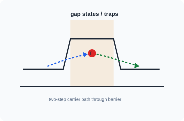
Dengeden sapıldığında (örneğin ışıkla fazla taşıyıcı üretildiğinde) sistem yeniden birleşme (rekombinasyon) yoluyla dengeye döner. Si gibi dolaylı yarı iletkenlerde baskın süreç, bant aralığı içindeki tuzak seviyeleri üzerinden gerçekleşen Shockley–Read–Hall (SRH) rekombinasyonudur. Azınlık taşıyıcılarının ortalama ömrü \(\tau\), difüzyon uzunluğu ise \(L = \sqrt{D\tau}\) ile verilir.
Tüm yarı iletken cihaz analizleri üç denklem grubuna dayanır: Poisson denklemi, akım yoğunluğu denklemleri (sürüklenme + difüzyon) ve süreklilik denklemleri. Sonraki haftalarda p-n eklemden transistörlere kadar tüm yapılar bu üçlüyle çözülecektir.
Sze karşılığı: Bölüm 1 (Physics and Properties of Semiconductors: A Review), kısım 1.2–1.7.
Akıllı telefon işlemcisi / SoC
Konu ile ilişkisi: Milyarlarca MOSFET'in çalışması Si kristal yapısı, katkılama, Fermi seviyesi ve taşıyıcı hareketliliğine dayanır. Bu haftadaki kristal yapı, enerji bantları, katkılama ve taşıyıcı hareketliliği kavramları doğrudan transistorun eşik gerilimini, kanal direncini ve anahtarlama hızını belirler; işlemci performansı bu mikroskobik özelliklerin milyarlarca elemanda kontrollü biçimde tekrarlanmasına dayanır.
Hangi cihazlarda: Akıllı telefonlar, tabletler, dizüstüler, yönlendiriciler ve giyilebilir cihazlardaki ana işlemci çiplerinde.
Ne amaçla kullanılır: Hesaplama, grafik, yapay zekâ ve sistem kontrolünü milyarlarca transistorla gerçekleştirmek.
Faydası: Çok yüksek entegrasyonla yüksek performans ve düşük enerji/işlem sağlar.
Dezavantaj / sınırlama: Düğüm küçüldükçe sızıntı, ısı yoğunluğu ve üretim maliyeti artar; küçük kusurlar bile yield'i düşürebilir.
Cihaz / yapı: İleri CMOS (FinFET/GAA sınıfı)
Göreli maliyet:Çok yüksek
Yaygın üretim yöntemi: 300 mm Si wafer; fotolitografi (ileri düğümlerde EUV + DUV), iyon implantasyonu/epitaksi, ince film biriktirme, aşındırma, CMP ve çok katmanlı metal bağlantılar
Ana maliyet sürücüsü: İleri litografi, maske setleri, çok sayıda proses adımı ve verim (yield)
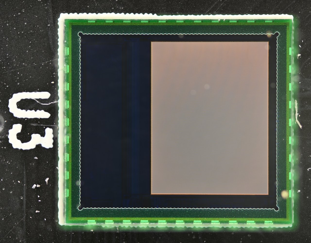
CMOS kamera sensörü
Konu ile ilişkisi: Piksellerdeki fotodiyotlar fotonları elektron–hol çiftlerine dönüştürür; bant aralığı ve yeniden birleşme duyarlılığı belirler. Buradaki bant aralığı, optik üretim–yeniden birleşme ve taşıyıcı ömrü kavramları pikselin hangi dalga boylarına duyarlı olduğunu, karanlık akımı ve düşük ışık performansını belirler; yani temel yarıiletken fiziği doğrudan görüntü kalitesine dönüşür.
Hangi cihazlarda: Akıllı telefon, dijital kamera, araç kamerası, güvenlik kamerası ve makine görüşü sistemlerinde.
Ne amaçla kullanılır: Işığı piksel başına elektrik yüküne dönüştürerek görüntü oluşturmak.
Faydası: Düşük güçle yüksek çözünürlük ve okuma elektroniğiyle aynı çipte entegrasyon sağlar.
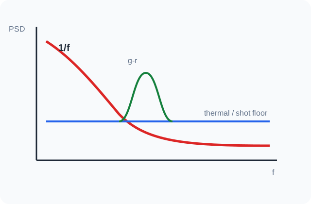
Dezavantaj / sınırlama: Karanlık akım, shot/1-f gürültüsü, doygunluk ve sıcaklık görüntü kalitesini sınırlar.
Cihaz / yapı: BSI CMOS görüntü sensörü + fotodiyot dizisi
Göreli maliyet:Yüksek
Yaygın üretim yöntemi: CMOS wafer işlemleri, fotodiyot implantları, metal katmanlar; modern BSI yapılarda wafer inceltme/bağlama, renk filtresi ve mikrolens
Ana maliyet sürücüsü: Piksel küçültme, wafer bonding, optik katmanlar ve test
GaN hızlı şarj adaptörü
Konu ile ilişkisi: Geniş bant aralıklı yarıiletkenler yüksek alan, sıcaklık ve hızlı anahtarlama gerektiren güç elektroniğinde avantaj sağlar. Bu örnek, bant aralığının yalnızca teorik bir enerji farkı olmadığını gösterir: geniş bant aralığı daha yüksek kritik elektrik alan ve sıcaklık dayanımı sağlar; bunun sonucu daha küçük, hızlı ve verimli güç dönüştürücüleridir.
Hangi cihazlarda: USB-C telefon/laptop şarj cihazları, kompakt adaptörler ve bazı yüksek frekanslı güç kaynaklarında.
Ne amaçla kullanılır: Şebeke veya DC gerilimi yüksek frekansta anahtarlayarak daha küçük ve verimli güç dönüşümü yapmak.
Faydası: Daha yüksek anahtarlama frekansı sayesinde trafo ve pasifler küçülür, verim artabilir.
Dezavantaj / sınırlama: GaN aygıtlar maliyetli olabilir; hızlı dv/dt EMI'yi artırır ve sürme/paket tasarımı daha hassastır.
Cihaz / yapı: GaN HEMT / GaN güç IC
Göreli maliyet:Yüksek
Yaygın üretim yöntemi: Genellikle GaN-on-Si epitaksi; heteroyapı büyütme, kapı ve ohmik kontak üretimi, pasivasyon ve güç paketleme
Ana maliyet sürücüsü: Epitaksi kalitesi, wafer verimi ve yüksek frekanslı paketleme
🏭 Ortak üretim referansı
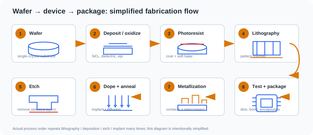
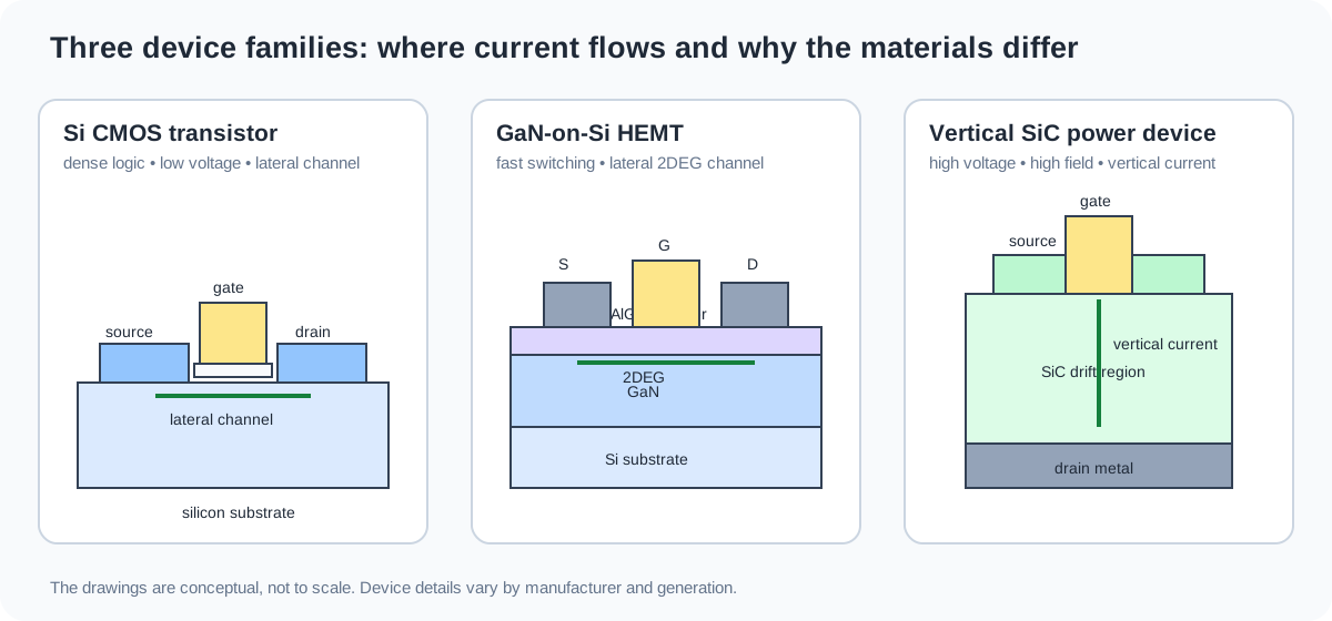
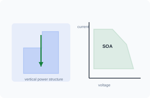
Wafer → litografi → aşındırma/katkılama → metalizasyon → test ve paketleme.Si CMOS, GaN HEMT ve dikey SiC güç aygıtlarında akım yolunun karşılaştırması.
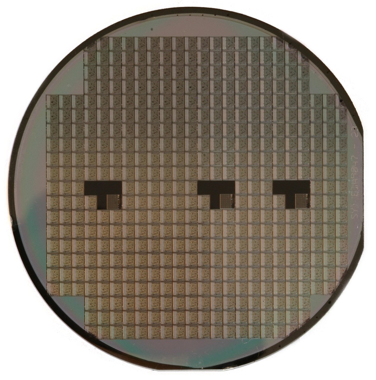
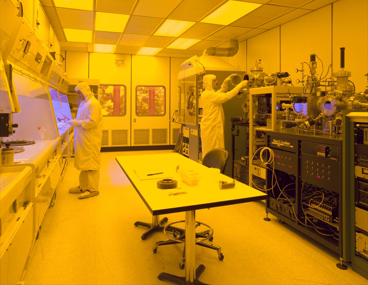
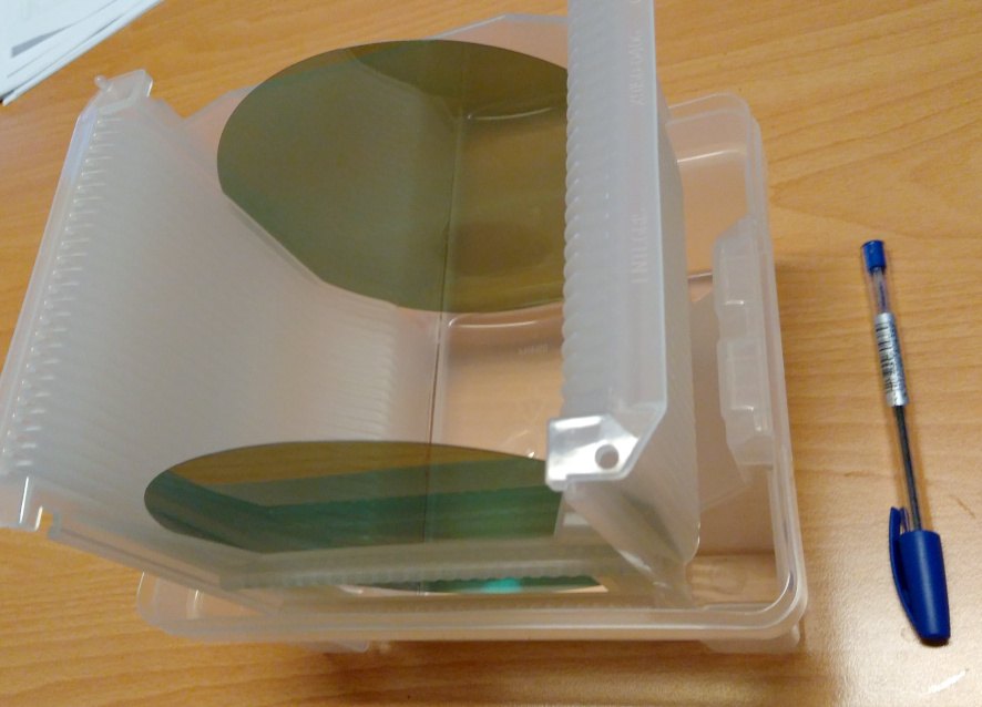
Silisyum wafer üzerinde çok sayıda entegre devre kalıbı · Inductiveload · Public DomainYarıiletken üretim temiz odası · NASA Glenn Research Center · Public Domain
Smartphone processor / SoC
Relation to this topic: Billions of MOSFETs rely on silicon crystal structure, doping, Fermi level and carrier mobility. The crystal structure, energy bands, doping and mobility studied this week directly set transistor threshold, channel resistance and switching speed; processor performance depends on reproducing these microscopic properties consistently across billions of devices.
Found in: Inside main processor chips in smartphones, tablets, laptops, routers and wearables.
Purpose: To perform computation, graphics, AI and system control using billions of transistors.
Benefit: Very high integration delivers high performance with low energy per operation.
Limitation / downside: As nodes shrink, leakage, heat density and fabrication cost rise; tiny defects can reduce yield.
Common manufacturing route: 300-mm silicon wafers; photolithography (EUV + DUV at advanced nodes), implantation/epitaxy, thin-film deposition, etch, CMP and multilayer interconnect
Main cost driver: Advanced lithography, mask sets, process count and yield
CMOS camera sensor
Relation to this topic: Pixel photodiodes convert photons into electron–hole pairs; bandgap and recombination influence sensitivity. Bandgap, optical generation–recombination and carrier lifetime determine wavelength sensitivity, dark current and low-light response. Fundamental semiconductor physics therefore becomes a direct image-quality limitation.
Found in: In smartphones, digital cameras, automotive cameras, security cameras and machine-vision systems.
Purpose: To convert incoming light into pixel-level electrical charge and form an image.
Benefit: Combines high resolution, low power and on-chip readout integration.
Limitation / downside: Dark current, shot/1-f noise, saturation and temperature limit image quality.
Common manufacturing route: CMOS wafer processing, photodiode implants and interconnect; modern BSI adds wafer thinning/bonding, color filters and microlenses
Main cost driver: Pixel scaling, wafer bonding, optical layers and test
GaN fast charger
Relation to this topic: Wide-bandgap semiconductors are advantageous where high electric field, temperature and fast switching are required. This example shows that bandgap is not merely an abstract energy difference: a wide bandgap supports higher critical electric field and temperature, enabling smaller, faster and more efficient power conversion.
Found in: In USB-C phone/laptop chargers, compact adapters and some high-frequency power supplies.
Purpose: To switch power at high frequency for smaller and more efficient conversion.
Benefit: Higher switching frequency can shrink transformers/passives and improve efficiency.
Limitation / downside: GaN can cost more; fast dv/dt increases EMI and demands careful gate-drive/package design.
Device / structure: GaN HEMT / GaN power IC
Relative cost:High
Common manufacturing route: Typically GaN-on-Si epitaxy; heterostructure growth, gate and ohmic contacts, passivation and power packaging
Main cost driver: Epitaxy quality, wafer yield and high-frequency packaging
🏭 Common manufacturing reference
Wafer → lithography → etch/doping → metallization → test and packaging.Comparison of current paths in Si CMOS, GaN HEMT and vertical SiC power devices.
Silicon wafer carrying many IC dies · Inductiveload · Public DomainSemiconductor manufacturing cleanroom · NASA Glenn Research Center · Public Domain
Bant kenarında parabolik yaklaşım ve etkin kütle
\[ E(\mathbf{k}) = E_C + \frac{\hbar^2 k^2}{2 m_n^*}, \qquad \frac{1}{m^*} = \frac{1}{\hbar^2}\frac{d^2E}{dk^2} \]Etkin kütle, \(E(k)\) eğrisinin eğriliğidir: dar (sivri) bant → küçük \(m^*\) → yüksek hareketlilik.
Aynı işlem valans bandındaki boş durumlar \(1-F(E)\) için yapılırsa \(p = N_V \exp[-(E_F - E_V)/kT]\) elde edilir.
\[ n = N_C\, e^{-(E_C-E_F)/kT}, \qquad p = N_V\, e^{-(E_F-E_V)/kT} \]Si, 300 K: \(N_C = 2.86\times10^{19}\), \(N_V = 2.66\times10^{19}\ \text{cm}^{-3}\). Her iki büyüklük de \(T^{3/2}\) ile ölçeklenir.
\[ E_i = \frac{E_C+E_V}{2} + \frac{kT}{2}\ln\frac{N_V}{N_C}, \qquad n = n_i\, e^{(E_F-E_i)/kT},\quad p = n_i\, e^{(E_i-E_F)/kT} \]\(E_i\), bant aralığının ortasından yalnızca birkaç meV sapar.
Yük nötrlüğü ve katkı iyonlaşması
\[ n + N_A^- = p + N_D^+ \]Sol taraf negatif, sağ taraf pozitif yükleri sayar. \(N_D^+\) ve \(N_A^-\) sabit (hareketsiz) iyonlardır; \(n\) ve \(p\) hareketli taşıyıcılardır.
\[ N_D^+ = \frac{N_D}{1 + g_D\,e^{(E_F-E_D)/kT}}, \qquad N_A^- = \frac{N_A}{1 + g_A\,e^{(E_A-E_F)/kT}} \]Taban durumu dejenerelik çarpanları Si için \(g_D=2\), \(g_A=4\). İyonlaşma enerjileri: P 45, As 54, Sb 39 meV (\(E_C-E_D\)); B 45, Al 67, Ga 72 meV (\(E_A-E_V\)).
Türetim: tam iyonlaşmada \(n\) ve \(p\)
\(N_D^+=N_D\), \(N_A^-=N_A\) ve \(p=n_i^2/n\) nötrlük denklemine yazılırsa:
Türetim: kompanzasyonsuz n tipinde freeze-out yaklaşımı
Çok düşük sıcaklıkta \(p\approx0\), \(N_A=0\) ve donörlerin çoğu nötrdür (\(e^{(E_F-E_D)/kT}\gg1\)). Nötrlük \(n = N_D^+\approx (N_D/g_D)\,e^{(E_D-E_F)/kT}\) olur. Bunu \(n=N_C e^{-(E_C-E_F)/kT}\) ile çarpıp \(E_F\)'yi yok edersek:
\[ \frac{1}{\mu}=\frac{1}{\mu_L}+\frac{1}{\mu_I},\qquad \mu_L\propto T^{-3/2},\qquad \mu_I\propto\frac{T^{3/2}}{N_I} \]Matthiessen kuralı: bağımsız saçılma oranları toplanır. \(\mu\), \(\mu_L=\mu_I\) sıcaklığında en büyük değerine ulaşır; bu sıcaklık \(N_I^{1/3}\) ile artar.
Türetim: Drude modeliyle \(\mu=q\tau_m/m^*\)
Bir taşıyıcı son saçılmadan sonra rastgele bir hızla yola çıkar; ortalaması sıfırdır. Sonraki \(t\) süresi boyunca alan ona \(\Delta v=-q\mathcal{E}t/m^*\) (elektron için) kazandırır. Saçılmalar arası süre üstel dağılımlı ve ortalaması \(\tau_m\) olduğundan \(\langle t\rangle=\tau_m\):
Hol için işaret pozitiftir. Saçılma ne kadar sıksa (\(\tau_m\) küçük) veya etkin kütle ne kadar büyükse hareketlilik o kadar düşer.
Neden \(\mu_L\propto T^{-3/2}\) ve \(\mu_I\propto T^{3/2}\)?
Fonon: Akustik fonon sayısı \(\propto T\), taşıyıcının saçılabileceği durum sayısı ve hızı \(\propto T^{1/2}\) ile artar: \(1/\tau_L\propto T\cdot T^{1/2}=T^{3/2}\).
İyonlaşmış katkı: Rutherford saçılmasında sapma açısı \(\propto 1/(m^*v^2)\); saçılma kesit alanı \(\propto v^{-4}\) ve oran \(\propto N_I\,v\,\sigma\propto N_I v^{-3}\). \(v\propto T^{1/2}\) konursa \(1/\tau_I\propto N_I T^{-3/2}\).
SRH rekombinasyonu
\[ U = \frac{\sigma_n\sigma_p v_{th} N_t\,(pn - n_i^2)}{\sigma_n\!\left[n + n_i e^{(E_t-E_i)/kT}\right] + \sigma_p\!\left[p + n_i e^{(E_i-E_t)/kT}\right]} \]Düşük enjeksiyonda n tipi malzeme için \(U \approx (p_n - p_{n0})/\tau_p\), \(\tau_p = 1/(\sigma_p v_{th} N_t)\). Rekombinasyon en etkili olarak \(E_t \approx E_i\) olduğunda gerçekleşir.
\(t=0\)'da \(x=0\)'a birim alan başına \(N\) adet fazla hol enjekte edilirse, \(G_p = 0\) ve düzgün \(\mathcal{E}\) altında süreklilik denkleminin çözümü:
Paket \(v = \mu_p\mathcal{E}\) hızıyla sürüklenir, \(\sqrt{2D_p t}\) genişliğiyle yayılır ve \(e^{-t/\tau_p}\) ile söner. Bu deney hareketlilik ve difüzyon katsayısını doğrudan ölçmeyi sağlar. Görseller sekmesinde canlandırmasını bulabilirsiniz.
Renk kodu tüm derste sabittir: mavi elektron ve iletim bandı, kırmızı hol ve valans bandı, yeşil Fermi seviyesi.
Elmas ve çinko sülfür birim hücresi (3B)
Fareyle döndürün. İki fcc alt örgünün iç içe geçtiğini ve her atomun dört komşusuyla dört yüzlü bağ kurduğunu görün. Zincblende modunda alt örgüler farklı renklenir (Ga/As).
E(k) yüzeyi: doğrudan ve dolaylı bant aralığı (3B)
İki boyutlu \(k\)-uzayında iletim ve valans bandı yüzeyleri. Dolaylı modda iletim bandı minimumu \(k \neq 0\)'a kayar: foton tek başına bu geçişi sağlayamaz, fonon gerekir.
Bant aralığı ölçeği: malzemeler, 1 eV ve \(kT\)
Logaritmik enerji ekseninde farklı malzemelerin bant aralıkları. Gökkuşağı şeridi görünür ışık fotonlarının enerjisini, kesikli çizgi seçilen sıcaklıktaki ısıl enerji \(kT\)'yi gösterir. Sıcaklığı değiştirin: \(kT\) bir malzemenin \(E_g\)'sine ne kadar yaklaşırsa o malzemede ısıl taşıyıcı o kadar bol olur. Noktaların üzerine gelince kesim dalga boyu \(\lambda_c=1240/E_g\) ve \(E_g/kT\) görünür.
Kristalden banda: katkı atomları ve taşıyıcılar
Solda iki boyuta indirgenmiş Si örgüsü (her çizgi iki elektronlu bir kovalent bağ), sağda aynı durumun bant diyagramı. Tipi değiştirin: P atomunun 5. elektronu nereye gidiyor, B atomunun eksik bağı nasıl hol oluyor? Sıcaklığı düşürüp freeze-out'u, yükseltip kopan bağları görün. Taşıyıcı sayıları sembolik, alttaki değerler gerçek hesaptır.
Durum yoğunluğu × Fermi–Dirac = taşıyıcı dağılımı
Solda bant diyagramı ve \(F(E)\), sağda \(N(E)F(E)\) (elektron) ve \(N(E)[1-F(E)]\) (hol). \(E_F\)'yi kaydırın: taşıyıcı yoğunluklarından biri artarken diğerinin nasıl üstel azaldığını görün. Sıcaklık, dağılımın kuyruğunu genişletir.
Has taşıyıcı yoğunluğunun sıcaklıkla değişimi
\(n_i\) ile \(1000/T\) yarı-logaritmik eksende neredeyse doğrudur; eğim \(-E_g/2k\)'dır. Geniş bant aralıklı GaAs'ın neden yüksek sıcaklıkta daha iyi çalıştığını gösterir. Eğriler Varshni ve \(T^{3/2}\) bağıntılarıyla hesaplanmıştır.
Sıcaklıkla üç rejim: freeze-out → extrinsic → intrinsic
Donör katkılı Si'de elektron yoğunluğu, eksik iyonlaşmayı da içeren nötrlük denkleminden hesaplanır. \(N_D\)'yi artırın: extrinsic plato yükselir ve intrinsic geçiş daha yüksek sıcaklığa kayar. İyonlaşma enerjisini artırın: freeze-out bölgesi genişler.
❄️ Freeze-out
Düşük sıcaklıkta donörlerin önemli kısmı elektronunu tutar, bu yüzden \(n\ll N_D\). Sıcaklık arttıkça donörler iyonlaşır ve \(n\) hızla yükselir.
⚙️ Extrinsic
Donörler neredeyse tamamen iyonlaşmıştır, intrinsic üretim ise küçüktür. Taşıyıcı sayısını katkı belirler: \(n\approx N_D\). Aygıtların çalışma bölgesi burasıdır.
🔥 Intrinsic
\(n_i\) üstel olarak büyüyüp \(N_D\)'yi yakalar. Katkı baskınlığını kaybeder ve sonunda \(n\approx p\approx n_i\) olur. Donörler hâlâ vardır, yalnızca taşıyıcı sayısını artık onlar belirlemez.
Katkılama ve Fermi seviyesinin konumu
Katkı türünü ve yoğunluğunu değiştirin. Fermi seviyesi yük nötrlüğü denkleminden hesaplanır. Katkı \(n_i\)'ye yaklaştığında malzeme hasa, \(10^{18}\ \text{cm}^{-3}\)'ün üzerinde ise dejenere olmaya yaklaşır.
n tipi mi, p tipi mi? \(N_D\) ile \(N_A\) yarışı
Solda: \(N_A\)'yı sabit tutup \(N_D\)'yi süpürdüğümüzde elektron ve hol yoğunlukları. \(N_D=N_A\) çizgisinin solunda malzeme p tipi, sağında n tipidir. Çoğunluk taşıyıcısı arttıkça azınlığın aynı oranda azaldığına dikkat edin: iki eğri her yerde \(np=n_i^2\) ile birbirine bağlıdır. Sağda: aynı durumda Si atom yoğunluğu, katkı yoğunlukları ve hareketli taşıyıcı yoğunlukları logaritmik eksende yan yana. Katkının ne kadar seyreltik olduğunu ve \(N_D\) ile \(n\)'nin ne zaman aynı çubuk boyuna geldiğini görün.
Si'de hareketlilik ve özdirenç – katkı ilişkisi
Düşük katkıda fonon saçılması, yüksek katkıda iyonize safsızlık saçılması baskındır. Sağ eksen, n ve p tipi Si'nin 300 K özdirencini verir (Caughey–Thomas modeli).
Saçılma simülasyonu: elektron, hol, fonon ve foton
Taşıyıcılar ısıl hızla rastgele koşar, alan onları yavaşça bir yöne iter. Yeşil halka fonon saçılması (titreşen Si atomu), sarı halka iyonlaşmış katkı saçılmasıdır (Coulomb sapması). Sıcaklığı düşürün: atomlar sakinleşir, fonon saçılması azalır ama yavaşlayan taşıyıcılar iyonlar tarafından çok daha sert saptırılır. Işığı açın: her foton bir elektron–hol çifti üretir, çift bir süre sonra rekombine olur. Alan ve hızlar görünür olsun diye abartılmıştır.
Matthiessen kuralı: hareketlilik sıcaklıkla neden tepe yapar?
Yukarıdaki sıcaklık, katkı iyonu ve taşıyıcı seçimi bu grafiği de günceller (1 iyon ≈ \(10^{16}\ \mathrm{cm^{-3}}\) iyonlaşmış katkı). Düşük sıcaklıkta katkı iyonları, yüksek sıcaklıkta fononlar hareketliliği sınırlar; toplam \(\mu\) her zaman ikisinden küçüktür. λ değeri gerçek Si parametreleriyle hesaplanır.
Haynes–Shockley: sürüklenme, difüzyon ve rekombinasyon
n tipi Si'ye darbe halinde enjekte edilen hol paketi. Zamanı ilerletin: paket alanla sürüklenir, difüzyonla genişler, ömürle söner. Üç süreci aynı anda görmek süreklilik denkleminin terimlerini somutlaştırır.
1. Si'nin elmas yapısında bir atomun en yakın komşu uzaklığı nedir? temel
Çözümü göster
En yakın komşu, cisim köşegeninin dörtte biri uzaklıktadır: \(d = \dfrac{\sqrt3}{4}a = \dfrac{\sqrt3}{4}(5.431\ \text{Å}) = 2.35\ \text{Å}\).
2. Si'nin 300 K'deki atom yoğunluğunu hesaplayınız. temel
Çözümü göster
Elmas birim hücresinde 8 atom vardır (8 köşe × 1/8 + 6 yüz × 1/2 + 4 iç = 8):
Hayır. Katkısız malzemede termal dengedeki hareketli elektron (ve hol) yoğunluğudur. Si'de 300 K'de \(n_i\approx10^{10}\ \mathrm{cm^{-3}}\), atom yoğunluğu ise \(5\times10^{22}\ \mathrm{cm^{-3}}\); yani yaklaşık her \(5\times10^{12}\) atoma bir serbest elektron düşer.
4. Saf Si'de elektron oluşunca hol neden oluşur? temel
Çözümü göster
Elektron valans bandındaki dolu bir durumdan, yani bir kovalent bağdan ayrılır. Arkasında bir elektron eksikliği bırakır; bu eksiklik hol olarak hareket eder. Bu yüzden saf malzemede \(n=p\).
5. Hol gerçek bir parçacık mıdır? kavramsal
Çözümü göster
Temel parçacık değildir. Valans bandındaki çok sayıda elektronun kolektif hareketini, tek bir boş durumun ters yönde hareketi olarak modellemek çok daha kolaydır. Bu boş durum \(+q\) yüklü ve pozitif etkin kütleli bir yarı-parçacık gibi davranır.
6. Si'ye \(N_D=10^{16}\ \mathrm{cm^{-3}}\) fosfor ekleniyor. Kaç Si atomuna bir P düşer? 300 K'de \(n\), \(p\) ve \(E_C-E_F\) nedir? orta
Çözümü göster
\[ \frac{5\times10^{22}}{10^{16}} = 5\times10^{6}\ \text{Si atomuna bir P}. \]
\(N_D \gg n_i\) olduğu için \(n \approx N_D = 10^{16}\ \text{cm}^{-3}\).
Dikkat: Taşıyıcı yoğunluğu net katkıya, hareketlilik ise toplam katkıya bağlıdır. Sık yapılan hata budur.
10. n tipi silisyum negatif yüklü müdür? kavramsal
Çözümü göster
Hayır. Her iyonlaşmış donör bir serbest elektron ve bir sabit \(\mathrm{P^+}\) iyonu üretir; toplam yük sıfırdır. Nötrlük \(n+N_A^-=p+N_D^+\) denklemiyle ifade edilir. “n tipi” ifadesi yalnızca çoğunluk taşıyıcısının negatif yüklü olduğunu söyler.
11. Si'de \(E_i\) bant aralığının ortasından ne kadar sapar? (300 K, \(N_C = 2.86\times10^{19}\), \(N_V = 2.66\times10^{19}\)) orta
Sapma 1 meV'dan küçüktür; pratikte \(E_i\) bant ortasında kabul edilir.
12. \(N_D=10^{15}\ \mathrm{cm^{-3}}\) Si yaklaşık hangi sıcaklıkta intrinsic davranmaya başlar? orta
Çözümü göster
Geçiş kabaca \(n_i(T)\approx N_D\) olduğunda başlar. \(n_i=\sqrt{N_C N_V}(T/300)^{3/2}e^{-E_g(T)/2kT}\) sayısal olarak çözülürse \(n_i=10^{15}\ \mathrm{cm^{-3}}\) yaklaşık 545 K'de sağlanır (\(N_D=10^{16}\) için ~650 K). Görseller sekmesindeki rejim grafiğinde \(N_D\)'yi değiştirerek bu kaymayı görebilirsiniz.
13. Çok düşük sıcaklıkta neden \(n<N_D\) olur? kavramsal
Çözümü göster
Donör elektronunu serbest bırakmak için yaklaşık 45 meV gerekir. \(kT\) bu enerjiye göre çok küçük olduğunda (ör. 30 K'de \(kT\approx2.6\) meV) elektronların çoğu donör atomuna bağlı kalır. Bu duruma freeze-out (donma) denir.
14. Yüksek sıcaklıkta n tipi etiketi neden anlamını yitirir? kavramsal
Çözümü göster
Termal elektron–hol üretimi, yani \(n_i\), üstel olarak artar ve donörlerin sağladığı taşıyıcı yoğunluğunu aşar. Bu durumda \(n\approx p\approx n_i\) olur ve malzemenin davranışını katkı değil sıcaklık belirler. Geniş bant aralıklı malzemelerin (SiC, GaN) yüksek sıcaklıkta tercih edilmesinin nedeni budur.
15. Hareketliliği \(\mu_p = 400\ \text{cm}^2/\text{V·s}\) olan hollerin 300 K'deki difüzyon katsayısı ve \(\tau_p = 1\ \mu\text{s}\) için difüzyon uzunluğu nedir? temel
16. Çarpışma ile saçılma arasındaki fark nedir? Mükemmel bir kristalde elektron saçılır mı? kavramsal
Çözümü göster
“Çarpışma” olayın gündelik adıdır ve temas imgesi taşır; “saçılma”, taşıyıcının momentumunun periyodikliği bozan bir etki yüzünden değişmesidir ve temas gerektirmez. Mükemmel, titreşmeyen bir kristalde elektron Bloch dalgası olarak saçılmadan ilerler; direnç fononlardan ve kusurlardan gelir.
17. \(\mu_n=1400\ \mathrm{cm^2/V\,s}\), \(m^*=0.26\,m_0\) olan Si elektronları için 300 K'de \(\tau_m\) ve ortalama serbest yol nedir? orta
Bu, Si atomları arasındaki ~0.24 nm mesafenin yaklaşık 200 katıdır.
18. Katkılı Si'yi 300 K'den 77 K'e soğutunca hareketlilik neden bazen artar, bazen azalır? orta
Çözümü göster
Soğutma fononları azaltır (\(\mu_L\) artar) ama taşıyıcıları yavaşlatır ve iyonlaşmış katkı saçılmasını güçlendirir (\(\mu_I\) azalır). Matthiessen kuralına göre hangisi daha küçükse o baskın olur: hafif katkılı Si'de \(\mu\) artar, yoğun katkılı Si'de iyon saçılması baskınlaşıp \(\mu\) azalabilir.
19. Si'ye ışık düşünce foton ve fonon ne rol oynar? kavramsal
Çözümü göster
\(h\nu\ge E_g\) olan foton soğurulur ve bir elektron–hol çifti üretir. Si dolaylı bant aralıklı olduğundan bant kenarı geçişinde momentumu bir fonon sağlar. Oluşan taşıyıcılar fononlarla saçılarak fazla enerjilerini ısı olarak örgüye verir, sonra çoğunlukla tuzaklar üzerinden rekombine olur; bu enerji de büyük ölçüde fonon (ısı) olarak açığa çıkar.
20. Neden Si'den verimli bir LED yapılamaz, GaAs'tan yapılabilir? kavramsal
Çözümü göster
Fotonun momentumu elektron momentumuna göre ihmal edilebilecek kadar küçüktür, bu yüzden optik geçişler \(E(k)\) diyagramında dikeydir. GaAs'ta bant uçları aynı \(k\)'dadır ve ışımalı geçiş doğrudan olur. Si'de iletim bandı minimumu ~0.85·(2π/a) noktasındadır; geçiş için bir fononun momentum sağlaması gerekir. Bu ikinci mertebe bir süreçtir, olasılığı çok düşüktür ve ışımasız SRH rekombinasyonu baskın hale gelir.
21. Isıl dengedeki bir Si parçasında taşıyıcılar hareket ettiği hâlde neden akım yoktur? kavramsal
Çözümü göster
Taşıyıcılar ~\(10^7\) cm/s ısıl hızla hareket eder ama yönleri rastgeledir; ortalama hızları sıfırdır. Akım için net bir yön gerekir: alan (sürüklenme), yoğunluk farkı (difüzyon) veya sıcaklık farkı. Isıl dengede bunların hiçbiri net etki üretmez; bir p-n ekleminde olduğu gibi alan olsa bile sürüklenme difüzyonla tam dengelenir.
22. Sabit ışık altındaki bir güneş hücresi ısıl dengede midir? \(np=n_i^2\) geçerli midir? orta
Çözümü göster
Hayır. Değerler zamanla değişmiyorsa hücre kararlı durumdadır, ama dışarıdan sürekli foton enerjisi aldığı için ısıl dengede değildir. Optik üretim fazla elektron ve hol yarattığından \(np>n_i^2\) olur; tek bir Fermi seviyesi yerine elektronlar ve holler için ayrı yarı-Fermi seviyeleri tanımlanır. Işık kesildiğinde fazla taşıyıcılar ömür \(\tau\) içinde rekombine olur ve hücre dengeye döner.
🎯 Bu hafta ne öğreneceğiz?
PN ekleminin tükenim bölgesinin neden oluştuğunu açıklamak.
Difüzyon ve sürüklenme akımlarının dengedeki ilişkisini kurmak.
Katkılama ile tükenim genişliği arasındaki ilişkiyi tahmin etmek.
🎯 Learning goals
Explain why the depletion region forms in a PN junction.
Relate diffusion and drift currents at equilibrium.
Predict how doping changes depletion width.
🧪 Önce tahmin et
N_A veya N_D artırıldığında tükenim bölgesinin hangi tarafa doğru daralacağını tahmin edin; sonra grafikte sınayın.
🧪 Predict first
Predict how increasing N_A or N_D changes each side of the depletion region, then test it on the graph.
⚠️ Sık yapılan hata
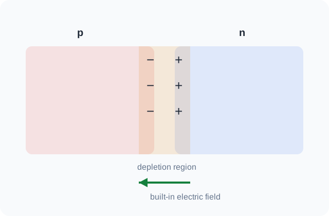
Tükenim bölgesi tamamen 'yüksüz' değildir. Serbest taşıyıcılardan tükenmiştir; geride iyonlaşmış katkı atomlarının uzay yükü kalır.
⚠️ Common misconception
The depletion region is not charge-free. It is depleted of mobile carriers while fixed ionized dopants remain.
p-n eklemi, tükenim bölgesi ve yerleşik elektrik alan · Özgün teknik şema
2.1 Eklemin oluşumu ve ısıl denge
p tipi ve n tipi iki yarı iletken tek bir kristal içinde yan yana getirildiğinde, ara yüzeyin iki tarafında taşıyıcı yoğunlukları arasında çok büyük bir fark oluşur. n tarafındaki elektronlar p tarafına, p tarafındaki holler n tarafına doğru difüzyonla geçer. Geride kalan iyonlaşmış katkı atomları hareket edemez: n tarafında pozitif verici iyonları, p tarafında negatif alıcı iyonları kalır. Bu sabit yükler bir uzay yükü bölgesi ve bu bölgede n'den p'ye yönelen bir iç elektrik alan oluşturur.
Oluşan alan, taşıyıcıları difüzyona zıt yönde sürükler. Isıl dengede her taşıyıcı türü için sürüklenme ve difüzyon akımları birbirini tam olarak dengeler ve net akım sıfırdır. Bunun matematiksel karşılığı, Fermi seviyesinin bütün yapı boyunca sabit olmasıdır. İki taraftaki \(E_F\) hizalanırken bantlar bükülür. İki bölge arasındaki elektrostatik potansiyel farkına yerleşik (built-in) potansiyel \(V_{bi}\) denir.
Sık karıştırılan nokta: Yerleşik potansiyel bir voltmetreyle ölçülemez. Metal kontaklardaki temas potansiyelleri \(V_{bi}\)'yi tam olarak dengeler, dış devrede gerilim görülmez.
2.2 Tükenim yaklaşımı ve ani eklem
Uzay yükü bölgesinde taşıyıcı yoğunlukları katkı yoğunluğuna göre ihmal edilebilecek kadar küçüktür. Tükenim yaklaşımında bu bölgenin serbest taşıyıcıdan tamamen arındığı, dışındaki bölgelerin ise tamamen nötr olduğu kabul edilir. Katkının ara yüzeyde basamak şeklinde değiştiği yapıya ani (abrupt) eklem denir.
Poisson denklemi bu bölgede kolayca integre edilir. Elektrik alan iki taraf boyunca doğrusal değişir ve maksimum değerine metalurjik eklemde ulaşır. Potansiyel ise parabolik değişir. Yük nötrlüğü gereği iki taraftaki toplam yük eşittir, \(N_A x_p = N_D x_n\). Bu yüzden tükenim bölgesi az katkılı tarafa doğru genişler. Bir taraf diğerinden çok daha yoğun katkılıysa (örneğin p\(^+\)n eklem) tükenim neredeyse tamamen az katkılı taraftadır. Bu tek taraflı eklem durumunda cihazın özelliklerini tek bir katkı yoğunluğu \(N_B\) belirler.
2.3 Doğrusal değişimli eklem
Difüzyonla üretilen eklemlerde katkı yoğunluğu ara yüzeyde aniden değişmez, yaklaşık doğrusal bir eğimle değişir: \(N_D - N_A = a x\). Bu durumda yük yoğunluğu doğrusal, elektrik alan parabolik, potansiyel ise kübik değişir. Tükenim genişliği gerilimin karekökü yerine küpkökü ile büyür. Bu fark kapasitans ölçümlerinde doğrudan gözlenir ve eklem profilini ayırt etmek için kullanılır.
2.4 Dış gerilim altında tükenim bölgesi
p tarafına n tarafına göre pozitif gerilim uygulandığında (ileri kutuplama) engel yüksekliği \(q(V_{bi}-V)\)'ye düşer ve tükenim bölgesi daralır. Ters kutuplamada engel yükselir, bölge genişler. Gerilimin neredeyse tamamı yüksek dirençli tükenim bölgesine düşer, nötr bölgelerdeki gerilim düşümü ihmal edilir.
Dış gerilim uygulandığında sistem artık dengede değildir, tek bir Fermi seviyesi tanımlanamaz. Elektronlar ve holler için ayrı ayrı yarı-Fermi seviyeleri \(E_{Fn}\) ve \(E_{Fp}\) tanımlanır. Tükenim bölgesi boyunca bu iki seviye yaklaşık sabit kalır ve aralarındaki fark \(qV\)'dir. 3. haftada diyot akımını türetirken bu gözlemi eklem yasası adıyla kullanacağız.
2.5 Tükenim kapasitansı
Uygulanan gerilim değiştiğinde tükenim bölgesinin kenarlarındaki yük değişir. Bu, iki levhası tükenim bölgesinin sınırları olan paralel levhalı bir kondansatör gibi davranır: \(C = \varepsilon_s/W\). Ters kutuplamada \(W\) büyüdükçe kapasitans azalır. Bu özellikten gerilim kontrollü kapasitör (varaktör) olarak yararlanılır.
Ani eklemde \(1/C^2\) gerilimle doğrusal değişir. Doğrunun eğimi az katkılı taraftaki katkı yoğunluğunu, gerilim eksenini kestiği nokta ise \(V_{bi}\)'yi verir. Bu C–V yöntemi, yarı iletken üretiminde katkı profili ölçmenin standart yollarından biridir. Eğim yerine yerel türev alınırsa katkı yoğunluğunun derinlikle değişimi \(N(W)\) de çıkarılabilir.
Sze karşılığı: Bölüm 2.1 ve 2.2 (Depletion Region: abrupt junction, linearly graded junction, arbitrary doping profile).
Güneş paneli hücresi
Konu ile ilişkisi: p-n eklemindeki yerleşik elektrik alan, ışıkla üretilen elektron ve holleri ayırarak fotovoltaik gerilim oluşturur. Bu haftadaki yerleşik potansiyel ve tükenim bölgesi güneş hücresinin yük ayırma mekanizmasının kendisidir; eklemin katkı profili ve tükenim genişliği, fototaşıyıcıların toplanma olasılığını ve hücrenin gerilim/akım karakteristiğini etkiler.
Hangi cihazlarda: Çatı ve arazi tipi güneş panellerinde, taşınabilir solar şarj cihazlarında ve enerji santrallerinde.
Ne amaçla kullanılır: Güneş ışığını doğrudan elektrik enerjisine dönüştürmek.
Faydası: Hareketli parça olmadan uzun ömürlü ve ölçeklenebilir elektrik üretimi sağlar.
Dezavantaj / sınırlama: Verim sıcaklık, gölgelenme, rekombinasyon ve yüzey/temas kayıplarıyla düşer; alan gereksinimi yüksektir.
Cihaz / yapı: Kristal Si p-n / passivated-contact hücre (PERC/TOPCon sınıfı)
Göreli maliyet:Orta
Yaygın üretim yöntemi: Si wafer tekstürleme, difüzyon/iyon katkılama, pasivasyon katmanları, metalizasyon ve ateşleme; yüksek hacimli hat üretimi
Ana maliyet sürücüsü: Wafer kalınlığı, gümüş/metal tüketimi, verim ve hat hacmi
Telefon ortam ışığı / yakınlık sensörü
Konu ile ilişkisi: Ters kutuplu fotodiyodun tükenim bölgesi fototaşıyıcıları hızla toplar. Ters kutuplama tükenim bölgesini genişletir ve bölgedeki elektrik alanı güçlendirir; bu sayede ışıkla oluşan taşıyıcılar rekombine olmadan hızla toplanır. Derste hesaplanan tükenim genişliği sensör hızına ve duyarlılığına bağlanır.
Hangi cihazlarda: Telefon, tablet, dizüstü, kulaklık kutusu ve ekranlarda otomatik parlaklık/yakınlık algılamasında.
Ne amaçla kullanılır: Ortam ışık seviyesini veya yakındaki nesnenin geri yansıttığı ışığı algılamak.
Faydası: Çok düşük güçle ekran parlaklığı ve dokunmatik/arama davranışını otomatik optimize eder.
Dezavantaj / sınırlama: Güçlü ortam ışığı, optik sızıntı ve paket kirlenmesi ölçümü bozabilir.
Cihaz / yapı: Si fotodiyot + CMOS okuma devresi
Göreli maliyet:Düşük–Orta
Yaygın üretim yöntemi: Standart/özel CMOS ile fotodiyot implantı, metalizasyon ve optik pencere/filtreli paketleme
Ana maliyet sürücüsü: Sensör alanı, optik paket ve kalibrasyon
RF varaktör
Konu ile ilişkisi: Ters gerilimle değişen tükenim genişliği, eklem kapasitansını değiştirerek frekans ayarına olanak verir. Varaktörde bir p-n eklemi kondansatör gibi davranır: ters gerilim tükenim genişliğini, dolayısıyla eklem kapasitansını değiştirir. Dersteki C–V ilişkisi burada doğrudan elektronik frekans ayar elemanına dönüşür.
Hangi cihazlarda: Telefon RF ön-uçları, tuner'lar, VCO/PLL devreleri, televizyon ve haberleşme alıcılarında.
Ne amaçla kullanılır: Ters gerilimle ayarlanabilen kapasitans oluşturarak frekans seçimi ve elektronik tuning yapmak.
Faydası: Mekanik ayar olmadan hızlı ve küçük boyutlu frekans kontrolü sağlar.
Dezavantaj / sınırlama: Doğrusal olmayan C-V davranışı distorsiyon üretir; Q faktörü ve parazitikler yüksek frekansta sınırlayıcıdır.
Cihaz / yapı: Ters kutuplu Si p-n eklem
Göreli maliyet:Düşük
Yaygın üretim yöntemi: Planar Si prosesi; kontrollü katkı profili, implant/difüzyon, eklem oluşturma ve RF paketleme
Ana maliyet sürücüsü: Wafer alanı küçük; performansı katkı profili ve RF paket parazitikleri belirler
🏭 Ortak üretim referansı
Wafer → litografi → aşındırma/katkılama → metalizasyon → test ve paketleme.Si CMOS, GaN HEMT ve dikey SiC güç aygıtlarında akım yolunun karşılaştırması.
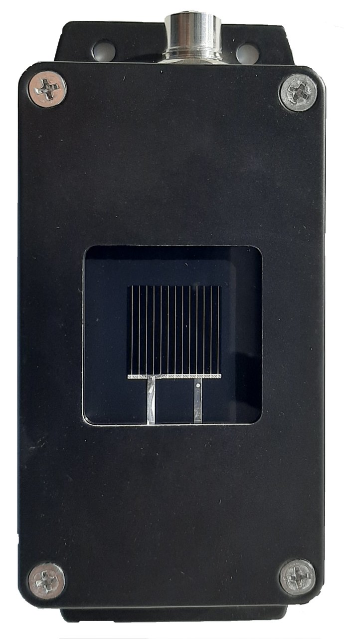
Referans silisyum güneş hücresi · Marta Victoria · CC BY-SA 4.0
Solar-panel cell
Relation to this topic: The built-in field of a p-n junction separates photogenerated electrons and holes to produce photovoltaic voltage. The built-in potential and depletion region studied this week are the solar cell's charge-separation mechanism. Junction doping and depletion width affect carrier collection and therefore the cell's voltage/current characteristic.
Found in: In rooftop/utility solar panels, portable solar chargers and photovoltaic plants.
Purpose: To convert sunlight directly into electrical energy.
Benefit: Long-lived, scalable generation with no moving parts.
Limitation / downside: Efficiency falls with temperature, shading, recombination and contact/surface losses; large area is required.
Common manufacturing route: Wafer texturing, diffusion/doping, passivation films, metallization and firing in high-volume lines
Main cost driver: Wafer use, metallization, efficiency and manufacturing scale
Phone ambient-light / proximity sensor
Relation to this topic: A reverse-biased photodiode uses its depletion region to collect photocarriers quickly. Reverse bias widens the depletion region and strengthens its electric field, allowing photocarriers to be swept out before recombination. The depletion width calculated in class thus maps directly to detector speed and sensitivity.
Found in: In phones, tablets, laptops, earbuds cases and displays for auto-brightness/proximity sensing.
Purpose: To measure ambient light or reflected light from a nearby object.
Benefit: Very low-power automatic control of display brightness and proximity behavior.
Limitation / downside: Strong ambient light, optical leakage and package contamination can distort readings.
Common manufacturing route: Standard/specialized CMOS with photodiode implants, interconnect and optically filtered packaging
Main cost driver: Sensor area, optical package and calibration
RF varactor
Relation to this topic: Reverse bias changes depletion width and therefore junction capacitance, enabling electronic frequency tuning. A varactor uses a p-n junction as a voltage-controlled capacitor: reverse voltage changes depletion width and hence junction capacitance. The class C–V relation becomes an electronic tuning mechanism.
Found in: In phone RF front ends, tuners, VCO/PLL circuits, TVs and communication receivers.
Purpose: To provide voltage-controlled capacitance for electronic frequency tuning.
Benefit: Fast, compact tuning without mechanical components.
Common manufacturing route: Planar silicon process with controlled doping profile, implantation/diffusion, junction formation and RF packaging
Main cost driver: Small die area; doping profile and package parasitics dominate
🏭 Common manufacturing reference
Wafer → lithography → etch/doping → metallization → test and packaging.Comparison of current paths in Si CMOS, GaN HEMT and vertical SiC power devices.
Reference silicon solar cell · Marta Victoria · CC BY-SA 4.0
Yerleşik potansiyel
Türetim: \(J_n = 0\) koşulundan \(E_F\) = sabit ve \(V_{bi}\)
Elektron akım yoğunluğu, \(n = n_i e^{(E_F-E_i)/kT}\) ve \(\mathcal{E} = \frac{1}{q}\frac{dE_i}{dx}\) kullanılarak tek bir terimde toplanabilir:
\[ V_{bi} = \frac{2kT}{q}\ln\frac{aW}{2n_i} \]\(V_{bi}\) ile \(W\) birbirine bağlıdır; ifade iteratif olarak çözülür (Görseller sekmesindeki hesap da böyle yapılır).
\[ \frac{1}{C_j^2} = \frac{2(V_{bi}-V)}{q\varepsilon_s N_B}, \qquad N(W) = \frac{2}{q\varepsilon_s}\left[-\frac{1}{d(1/C^2)/dV}\right] \]Genel profil için tükenim kenarındaki yük artışı \(dQ = qN(W)\,dW\) kullanılır; sonuç her derinlikteki yerel katkıyı verir.
Renk kodu: mavi elektron/iletim bandı, kırmızı hol/valans bandı, yeşil (yarı-)Fermi seviyesi.
Eklemin dört yüzü: yük, alan, potansiyel ve bant diyagramı
Dört grafik aynı \(x\) eksenini paylaşır ve birbirinin integralidir: yük → (∫) → alan → (−∫) → potansiyel → bant bükülmesi. Katkıları değiştirip tükenimin az katkılı tarafa kaydığını, gerilimi değiştirip yarı-Fermi seviyelerinin ayrışmasını izleyin. Yarı-Fermi seviyelerinin nötr bölgelerdeki sönümü şematiktir; gerçek difüzyon uzunlukları tükenim genişliğinden çok daha büyüktür.
İletim bandı kenarı \(E_C(x, V)\) yüzeyi (3B)
Aynı ani eklemin bant kenarı, tüm gerilim aralığı için tek bir yüzeyde. Ters kutuplama derinleştikçe basamağın yükseldiğini ve eğimli bölgenin (tükenim) genişlediğini görün. Genişleme \(\sqrt{V_{bi}-V}\) ile olduğu için yüzeyin kenarı parabolik bir iz çizer. Yukarıdaki \(N_A\), \(N_D\) kaydırıcıları bu yüzeyi de günceller.
C–V ölçümü: ani ve doğrusal değişimli eklem
p\(^+\)n eklem (\(N_A = 10^{19}\)) ve aynı sıfır-gerilim kapasitansına sahip doğrusal değişimli eklem. Sağda \(1/C^2\): ani eklem için düz bir doğru elde edilir, eğim \(N_D\)'yi, gerilim eksenini kestiği nokta \(V_{bi}\)'yi verir. Doğrusal eklemde eğri bükülür; bu bükülme profilin ani olmadığının işaretidir.
1. \(N_A = 10^{17}\), \(N_D = 10^{15}\ \text{cm}^{-3}\) olan bir Si ani ekleminin 300 K'deki yerleşik potansiyelini bulunuz. temel
\(2kT/q\) düzeltmesiyle \(W(0) = 0.93\ \mu\text{m}\) olur; ters kutuplamada düzeltme ihmal edilebilir.
3. Yukarıdaki eklemde tükenim bölgesinin yüzde kaçı n tarafındadır? Neden? temel
Çözümü göster
\(x_n/x_p = N_A/N_D = 100\), dolayısıyla \(x_n/W = 100/101 \approx \%99\). İki taraftaki toplam yük eşit olmak zorundadır. Az katkılı tarafta birim hacimdeki yük 100 kat küçük olduğundan, aynı yükü sağlamak için 100 kat daha geniş bir bölgenin tükenmesi gerekir.
4. \(-5\) V'ta birim alan başına kapasitans ve 100 μm × 100 μm'lik bir diyotun toplam kapasitansı nedir? temel
Çözümü göster
\[ C_j = \frac{\varepsilon_s}{W} = \frac{1.05\times10^{-12}}{2.74\times10^{-4}} = 3.84\ \text{nF/cm}^2, \qquad C = C_j A = 3.84\times10^{-9}\cdot10^{-4} = 0.38\ \text{pF}. \]
5. Bir p\(^+\)n Si diyotta ölçülen \(1/C^2\)–\(V\) doğrusunun eğimi \(-1.19\times10^{15}\ \text{cm}^4\,\text{F}^{-2}\,\text{V}^{-1}\), gerilim eksenini kestiği nokta 0.85 V'tur. \(N_D\) ve \(N_A\)'yı bulunuz. orta
Dikkat: \(N_A\) üstel ifadeyle hesaplandığından kesim noktasındaki 10 mV'luk bir hata \(N_A\)'da yaklaşık %50 hataya yol açar. C–V yöntemi az katkılı tarafı iyi, çok katkılı tarafı kötü ölçer.
6. Isıl dengede tükenim bölgesinde güçlü bir elektrik alan varken neden akım akmaz? kavramsal
Çözümü göster
Alan gerçekten taşıyıcıları sürükler, ancak aynı bölgede taşıyıcı yoğunluğu çok dik bir gradyana sahiptir ve buna bağlı difüzyon akımı tam ters yöndedir. Dengede iki akım her noktada birbirini sıfırlar; bu, \(J_n = \mu_n n\,dE_F/dx = 0\) ifadesiyle \(E_F\)'nin sabit olmasının anlamıdır. Her iki bileşen tek başına tipik olarak \(10^{3}\)–\(10^{4}\ \text{A/cm}^2\) mertebesindedir; diyot akımı bu iki büyük sayı arasındaki küçük dengesizlikten doğar.
🎯 Bu hafta ne öğreneceğiz?
Kutuplamanın enerji engelini ve azınlık taşıyıcı enjeksiyonunu nasıl değiştirdiğini açıklamak.
Shockley diyot davranışını fiziksel kökeniyle ilişkilendirmek.
İdeal modelin sınırlarını ayırt etmek.
🎯 Learning goals
Explain how bias changes the barrier and minority-carrier injection.
Connect Shockley diode behavior to its physical origin.
Recognize the limits of the ideal model.
🧪 Önce tahmin et
İleri gerilimi küçük bir miktar artırınca akımın neden doğrusal değil çok hızlı arttığını önce bant/taşıyıcı resmiyle açıklamaya çalışın.
🧪 Predict first
Before calculating, explain from the band/carrier picture why a small increase in forward voltage can cause a rapid, non-linear current increase.
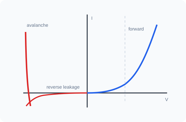
Gerçek diyot I–V eğrisi: ileri iletim, sızıntı ve kırılma · Özgün teknik şema
3.1 Kutuplama altında sınır koşulları
İleri kutuplamada engel yüksekliği \(qV\) kadar azalır. Tükenim bölgesinde sürüklenme ve difüzyon arasındaki büyük dengenin küçük bir kısmı bozulur ve taşıyıcılar karşı tarafa enjekte edilir. n bölgesine geçen holler orada azınlık taşıyıcısıdır; tükenim kenarındaki yoğunlukları denge değerinin \(e^{qV/kT}\) katına çıkar. Bu ilişkiye eklem yasası denir ve yarı-Fermi seviyelerinin tükenim bölgesinde sabit ve \(qV\) kadar ayrık olmasının doğrudan sonucudur.
Ters kutuplamada aynı yasa kenardaki azınlık taşıyıcı yoğunluğunun sıfıra yakın olduğunu söyler. Tükenim bölgesi, kenarına ulaşan azınlık taşıyıcılarını karşı tarafa süpürür; akımı sınırlayan, bu taşıyıcıların ne kadar hızlı üretilip kenara difüzyonla ulaşabildiğidir.
3.2 İdeal diyot: Shockley denklemi
Shockley modeli dört varsayıma dayanır: (1) tükenim bölgesi ani sınırlıdır ve dışında bölge nötrdür; (2) Boltzmann yaklaşımı geçerlidir; (3) düşük enjeksiyon: enjekte edilen azınlık yoğunluğu çoğunluk yoğunluğunun çok altındadır; (4) tükenim bölgesinde üretim ve yeniden birleşme olmaz, akımlar bu bölgede sabittir.
Bu varsayımlarla nötr bölgelerde alan sıfırdır ve azınlık taşıyıcıları yalnızca difüzyonla hareket eder. Süreklilik denklemi üstel sönen bir profil verir; fazla taşıyıcılar yaklaşık bir difüzyon uzunluğu \(L\) içinde yeniden birleşir. Tükenim kenarındaki difüzyon akımlarının toplamı diyot akımını verir. Sonuç, ileri yönde üstel artan, ters yönde doyum akımına \(-J_s\) oturan ünlü diyot denklemidir.
Akımın nötr bölgelerdeki yapısına dikkat edin: tükenim kenarında akım tamamen azınlık taşıyıcılarıyla taşınır. Kenardan uzaklaştıkça azınlık akımı yeniden birleşmeyle azalır, her yeniden birleşme olayı için karşı taraftan bir çoğunluk taşıyıcısı gelir. Toplam akım her yerde sabittir. Görseller sekmesindeki akım bileşenleri grafiği bu devri gösterir.
Tek taraflı p\(^+\)n eklemde \(n_{p0} = n_i^2/N_A\) ihmal edilecek kadar küçüktür ve akımı az katkılı taraftaki hol enjeksiyonu belirler. Az katkılı bölge difüzyon uzunluğundan kısaysa (kısa taban) \(L_p\) yerine bölge genişliği yazılır. Bu durum 9. haftada transistörün taban bölgesinde tekrar karşımıza çıkacak.
3.3 İdeal davranıştan sapmalar
Üretim akımı (ters yön)
Ters kutuplamada tükenim bölgesinde \(pn \ll n_i^2\) olur ve SRH süreci ters işleyerek taşıyıcı çifti üretir. Üretilen çiftler alanla hemen süpürülür. Bu akım \(n_i\) ile orantılıdır, ideal doyum akımı ise \(n_i^2\) ile. Si gibi \(n_i\)'si küçük malzemelerde oda sıcaklığında üretim akımı baskındır ve \(W\) ile birlikte büyüdüğü için ters akım doymaz, \(\sqrt{V}\) gibi artar.
Yeniden birleşme akımı (ileri yön, düşük gerilim)
İleri kutuplamada tükenim bölgesinde \(pn > n_i^2\) olur ve yeniden birleşme gerçekleşir. Yeniden birleşme hızı \(n\) ile \(p\)'nin eşit olduğu noktada en büyüktür; orada \(n = p = n_i e^{qV/2kT}\). Bu akım \(e^{qV/2kT}\) ile artar, yani ideallik faktörü 2'dir. Düşük gerilimlerde baskındır.
Yüksek enjeksiyon ve seri direnç
Enjekte edilen azınlık yoğunluğu çoğunluk yoğunluğuna yaklaştığında nötrlük korunmak için çoğunluk taşıyıcıları da artar, nötr bölgede küçük bir alan oluşur ve akım \(e^{qV/2kT}\) ile artmaya başlar. Daha yüksek akımlarda nötr bölgelerin ve kontakların direnci üzerindeki \(IR_s\) düşümü eklem gerilimini azaltır ve \(\log I\)–\(V\) eğrisi bükülür.
Bu etkilerin hepsi ideallik faktörü \(\eta\) ile özetlenir: \(I \propto e^{qV/\eta kT}\). \(\eta = 1\) difüzyonun, \(\eta \approx 2\) yeniden birleşmenin veya yüksek enjeksiyonun baskın olduğunu gösterir. Ölçülen bir \(\log I\)–\(V\) eğrisinin eğimi bu yüzden cihazın içinde hangi mekanizmanın çalıştığını söyler.
Sıcaklık etkisi
Doyum akımı \(n_i^2\) üzerinden sıcaklığa çok güçlü bağlıdır: Si'de oda sıcaklığı civarında her 10 K'de yaklaşık 4–5 kat artar. Sabit akımda ileri gerilim yaklaşık −2 mV/K ile azalır; bu özellik diyotları basit sıcaklık algılayıcıları olarak kullanılabilir kılar.
3.4 Eklem kırılması
Ters gerilim belirli bir değere ulaştığında akım aniden artar. Üç mekanizma vardır: ısıl kararsızlık (dar bant aralıklı malzemelerde), tünelleme ve çığ çoğalması.
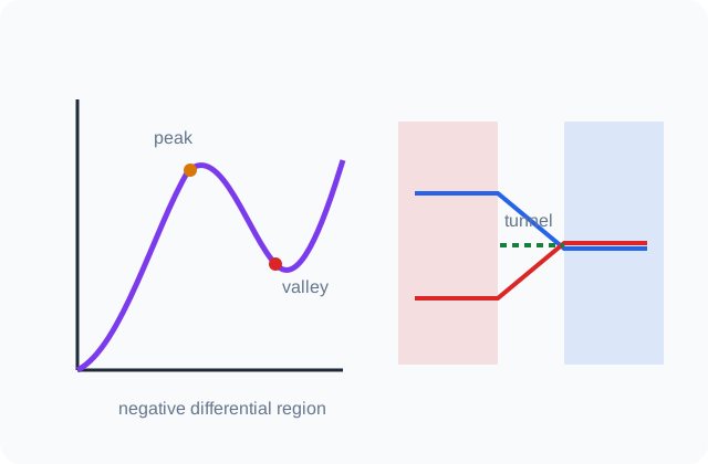
Tünelleme (Zener) kırılması çok yoğun katkılı eklemlerde görülür. Tükenim bölgesi o kadar dardır (~10 nm) ki elektronlar p tarafının valans bandından n tarafının iletim bandına kuantum mekaniksel olarak tünelleyebilir. Si'de kırılma gerilimi \(4E_g/q\)'dan küçükse mekanizma tünellemedir.
Çığ (avalanche) kırılması daha az katkılı eklemlerde baskındır. Alanla hızlanan bir taşıyıcı, bant aralığından fazla kinetik enerji kazanınca örgüye çarpıp yeni bir elektron-hol çifti koparır (darbe iyonlaşması). Yeni taşıyıcılar da hızlanıp çift üretir ve süreç çığ gibi büyür. Kırılma gerilimi \(6E_g/q\)'nun üzerindeyse mekanizma çığdır; aradaki bölgede ikisi birlikte etkilidir.
İki mekanizma sıcaklık katsayılarıyla ayırt edilir. Sıcaklık arttıkça bant aralığı küçülür ve tünelleme kolaylaşır: Zener gerilimi azalır. Aynı artış fonon saçılmasını da güçlendirir, taşıyıcılar iyonlaşma enerjisini kazanmakta zorlanır: çığ gerilimi artar. Yaklaşık 5–6 V'luk Zener diyotların sıcaklık katsayısının neredeyse sıfır olması bu iki etkinin birbirini dengelemesinden gelir.
Sze karşılığı: Bölüm 2.3 (Current–Voltage Characteristics), 2.4 (Junction Breakdown).
USB-C / HDMI ESD koruma diyodu
Konu ile ilişkisi: TVS diyotlar aşırı gerilim darbelerinde çığ kırılmasına girerek hassas girişleri sınırlar ve korur. Dersteki ters kutuplama ve çığ kırılması TVS diyodunun normal çalışma ilkesidir; kısa süreli yüksek gerilimde taşıyıcı çoğalması akımı üzerine alır ve hat gerilimini güvenli bir seviyede sınırlar. Kırılma fiziği bu nedenle doğrudan koruma performansını belirler.
Hangi cihazlarda: Telefon, laptop, TV, modem ve otomotiv elektroniklerinin USB, HDMI, Ethernet ve benzeri dış bağlantı uçlarında.
Ne amaçla kullanılır: ESD ve ani gerilim darbelerini hassas IC girişlerinden uzaklaştırıp toprağa boşaltmak.
Faydası: Ucuz ve hızlı bir koruma katmanı sağlayarak pahalı ana çiplerin arızalanmasını önler.
Dezavantaj / sınırlama: Ek kapasitans yüksek hızlı hatların sinyal bütünlüğünü bozabilir; yanlış seçilen klemp gerilimi korumayı zayıflatır.
Cihaz / yapı: Si TVS / avalanche junction
Göreli maliyet:Düşük
Yaygın üretim yöntemi: Planar Si eklem prosesi, kontrollü yüksek alan bölgesi, metalizasyon; çok kanallı dizilerde küçük paket entegrasyonu
Ana maliyet sürücüsü: Küçük kalıp alanı; paket ve test çoğu zaman önemli pay tutar
Zener gerilim referansı
Konu ile ilişkisi: Zener/çığ bölgesi, belirli bir gerilim çevresinde referans veya sınırlama elemanı olarak kullanılır. Zener/çığ bölgesindeki keskin I–V değişimi, akım değişse bile gerilimin yaklaşık sabit tutulmasını sağlar. Dersteki idealden sapma ve kırılma mekanizmaları, pratikte referans doğruluğu ve sıcaklık katsayısı olarak karşımıza çıkar.
Hangi cihazlarda: Güç yönetim IC'leri, ölçüm devreleri, basit regülatörler ve koruma devrelerinde.
Ne amaçla kullanılır: Kararlı bir referans veya gerilim klempi oluşturmak.
Faydası: Basit devreyle belirli bir gerilim eşiği elde etmeyi sağlar.
Dezavantaj / sınırlama: Dinamik direnç, sıcaklık katsayısı ve gürültü hassas uygulamalarda doğruluğu sınırlar.
Cihaz / yapı: Si Zener/çığ diyodu
Göreli maliyet:Düşük
Yaygın üretim yöntemi: Yüksek katkılı p-n eklem için implant/difüzyon, aktivasyon tavlaması, metalizasyon ve wafer-probe sınıflandırması
Ana maliyet sürücüsü: Basit proses ve küçük alan; hassas tolerans için test/sınıflandırma
Güç kaynağı doğrultucusu
Konu ile ilişkisi: İleri kutuplama, seri direnç ve yüksek enjeksiyon gerçek I–V eğrisini ve ısınmayı belirler. Shockley davranışı düşük/orta akımda iyi bir başlangıçtır; fakat gerçek güç diyodunda seri direnç, yüksek enjeksiyon ve ısınma baskınlaşır. Bu haftadaki ideal–gerçek farkı doğrudan iletim kaybı ve termal tasarıma dönüşür.
Hangi cihazlarda: Adaptör, SMPS, TV güç kartı, beyaz eşya ve endüstriyel güç kaynaklarında.
Ne amaçla kullanılır: AC'yi DC'ye doğrultmak veya anahtarlamalı güç devresindeki akım yolunu tek yönlü hale getirmek.
Faydası: Basit ve sağlam enerji yönlendirmesi sağlar.
Dezavantaj / sınırlama: İleri gerilim düşümü ve ters toparlanma kaybı ısı ve verim kaybına yol açar.
Cihaz / yapı: Si Schottky / hızlı p-n diyot
Göreli maliyet:Orta
Yaygın üretim yöntemi: Planar veya trench yapı; bariyer metali ya da p-n eklem üretimi, kalın metal ve düşük dirençli güç paketi
Ana maliyet sürücüsü: Akım taşıma alanı, termal paket ve düşük kayıplı metalizasyon
🏭 Ortak üretim referansı
Wafer → litografi → aşındırma/katkılama → metalizasyon → test ve paketleme.Si CMOS, GaN HEMT ve dikey SiC güç aygıtlarında akım yolunun karşılaştırması.
USB-C / HDMI ESD protection diode
Relation to this topic: TVS diodes enter avalanche breakdown during voltage transients to clamp and protect sensitive inputs. Reverse bias and avalanche breakdown are the normal operating physics of a TVS diode. During a transient, carrier multiplication diverts current and clamps the line; breakdown physics therefore determines protection performance.
Found in: On USB, HDMI, Ethernet and other exposed ports in phones, laptops, TVs, modems and cars.
Purpose: To divert ESD and transient overvoltage away from sensitive IC inputs.
Benefit: Adds a fast, inexpensive protection layer that can save much more expensive chips.
Limitation / downside: Added capacitance can degrade high-speed signal integrity; a poorly chosen clamp voltage weakens protection.
Common manufacturing route: Planar silicon junction process with controlled high-field region, metallization and compact multichannel packaging
Main cost driver: Small die; packaging and test can be a large share
Zener voltage reference
Relation to this topic: Zener/avalanche operation provides a useful voltage reference or clamp around a defined voltage. The steep I–V response in Zener/avalanche operation allows voltage to remain approximately fixed over a range of current. Non-ideal breakdown effects studied here appear in practice as reference accuracy and temperature coefficient.
Found in: In power-management ICs, measurement circuits, simple regulators and protection circuits.
Purpose: To create a stable reference or voltage clamp.
Benefit: Provides a useful voltage threshold with very simple circuitry.
Limitation / downside: Dynamic resistance, temperature coefficient and noise limit precision applications.
Device / structure: Silicon Zener/avalanche diode
Relative cost:Low
Common manufacturing route: Implant/diffusion for a heavily doped junction, activation anneal, metallization and wafer-level binning
Main cost driver: Simple process and small area; precision binning adds cost
Power-supply rectifier
Relation to this topic: Forward bias, series resistance and high injection shape the real I–V curve and heating. Shockley behavior is a useful low/moderate-current starting point, but series resistance, high injection and self-heating dominate real power diodes. The ideal-versus-real distinction becomes conduction loss and thermal design.
Found in: In adapters, SMPS units, TVs, appliances and industrial power supplies.
Purpose: To rectify AC to DC or enforce one-way current flow in switching converters.
Benefit: Simple and robust energy steering.
Limitation / downside: Forward drop and reverse-recovery loss create heat and reduce efficiency.
Device / structure: Silicon Schottky / fast p-n diode
Relative cost:Medium
Common manufacturing route: Planar or trench process; barrier metal or p-n junction formation, thick metal and low-resistance power package
Main cost driver: Current-carrying area, thermal package and low-loss metallization
🏭 Common manufacturing reference
Wafer → lithography → etch/doping → metallization → test and packaging.Comparison of current paths in Si CMOS, GaN HEMT and vertical SiC power devices.
Yarı-Fermi seviyeleri ve eklem yasası
\[ n = n_i\,e^{(E_{Fn}-E_i)/kT},\qquad p = n_i\,e^{(E_i-E_{Fp})/kT},\qquad pn = n_i^2\,e^{(E_{Fn}-E_{Fp})/kT} \]
p tarafı için aynı işlem \(J_n(-x_p)\)'yi verir. Tükenim bölgesinde üretim-yeniden birleşme olmadığından her iki akım bileşeni bu bölge boyunca sabittir; toplam akım \(J = J_p(x_n) + J_n(-x_p)\).
\[ T_t \approx \exp\!\left(-\frac{4\sqrt{2m^*}\,E_g^{3/2}}{3q\hbar\mathcal{E}}\right) \]Üçgen engelden tünelleme olasılığı (WKB). Zener kırılmasını ve 4. haftadaki tünel diyodu bu ifade yönetir.
Renk kodu: mavi elektron, kırmızı hol, yeşil toplam veya Fermi seviyesi.
Azınlık taşıyıcı profilleri ve akım bileşenleri
Si eklem: \(N_A = 10^{17}\), \(N_D = 10^{16}\), \(\tau = 1\ \mu\)s. Üstte logaritmik eksende taşıyıcı yoğunlukları, altta akımın elektron ve hol payı. İleri kutuplamada kenardaki azınlık yoğunluğunun \(e^{qV/kT}\) ile büyüdüğünü, ters kutuplamada ise kenarın boşaldığını izleyin. Alt grafik, azınlık akımının yeniden birleşmeyle çoğunluk akımına devredildiğini ve toplamın sabit kaldığını gösterir. Dar sarı şerit gerçek ölçekli tükenim bölgesidir.
Gerçek diyot I–V eğrisi ve bileşenleri
p\(^+\)n Si diyot, alan \(10^{-4}\ \text{cm}^2\). Kesikli çizgiler bileşenleri, kalın çizgi ölçülecek toplam akımı gösterir. Ömrü kısaltın: yeniden birleşme bileşeni (\(\eta = 2\)) büyür ve düşük gerilim bölgesini ele geçirir. Seri direnç yüksek akımda eğriyi yatırır. Sol taraf ters yöndür: akım doymaz, üretim akımı \(\sqrt{V}\) gibi artmaya devam eder.
log I(V, T) yüzeyi (3B)
Aynı diyotun ileri yön akımı, gerilim ve sıcaklığın fonksiyonu olarak (τ = 1 μs, \(R_s = 0\)). Sabit akım düzleminde (yatay kesit) sıcaklık arttıkça gerekli gerilimin azaldığını görün: yaklaşık −2 mV/K. Yüzey üzerindeki kontur çizgileri eşit akım eğrileridir.
Kırılma gerilimi ve mekanizma bölgeleri
Solda tek taraflı ani eklemler için \(V_B\)–\(N_B\) ilişkisi (Sze ampirik bağıntısı). Si için gri bant tünelleme ile çığ arasındaki geçiş bölgesidir (\(4E_g\)–\(6E_g\)). Sağda seçilen katkıda ters yön I–V eğrisi: çoğalma faktörü \(M\) kırılmaya yaklaşırken sonsuza gider.
1. Bir p\(^+\)n Si diyotta \(N_D = 10^{16}\ \text{cm}^{-3}\), \(\tau_p = 1\ \mu\)s, \(\mu_p = 429\ \text{cm}^2/\text{V·s}\), alan \(10^{-4}\ \text{cm}^2\)'dir. \(I_s\)'yi ve \(V = 0.6\) V'taki akımı bulunuz. temel
\(J_{gen}/J_s \approx 2.7\times10^{4}\). Si diyotta oda sıcaklığında ölçülen ters akım neredeyse tamamen üretim akımıdır. Oran \(N_D W/(n_i L_p)\) ile orantılı olduğundan sıcaklık artınca (\(n_i\) büyüyünce) difüzyon bileşeni öne geçer.
3. Bir diyotun ileri akımı düşük gerilimde her 118 mV'ta, orta gerilimde her 60 mV'ta on kat artıyor. Yorumlayınız. orta
Çözümü göster
\(\eta = \Delta V/59.5\ \text{mV}\): düşük gerilimde \(\eta \approx 2\) (tükenim bölgesinde yeniden birleşme baskın), orta gerilimde \(\eta \approx 1\) (ideal difüzyon akımı). Geçiş geriliminin düşük olması tuzak yoğunluğunun az, yani ömrün uzun olduğunu gösterir. Daha yüksek akımlarda eğrinin tekrar yatması yüksek enjeksiyon veya seri direnç işaretidir.
4. Si diyotun doyum akımı 300 K'den 310 K'e çıkınca kaç kat artar? (\(J_s \propto T^3e^{-E_g/kT}\), \(E_g = 1.12\) eV) orta
Kabaca her 5 K'de iki katına çıkar. Güç devrelerinde ısıl kaçak (thermal runaway) riskinin kaynağı budur (12. hafta).
5. \(N_B = 10^{16}\ \text{cm}^{-3}\) olan tek taraflı Si eklemde \(V_B\), kırılmadaki tükenim genişliği ve kritik alan nedir? Mekanizma hangisidir? orta
\(V_B \gg 6E_g/q = 6.7\) V olduğundan mekanizma çığ kırılmasıdır. \(W_m = 2.85\ \mu\text{m}\), tünelleme için gereken ~10 nm'den çok büyüktür.
6. 3.3 V'luk ve 12 V'luk iki Zener diyotun sıcaklık katsayılarının işaretleri nedir? Neden? kavramsal
Çözümü göster
3.3 V \(< 4E_g/q\): tünelleme mekanizmasıdır, sıcaklıkla \(E_g\) azaldığından tünelleme kolaylaşır, katsayı negatiftir. 12 V \(> 6E_g/q\): çığ mekanizmasıdır, sıcaklıkla fonon saçılması artar ve taşıyıcıların iyonlaşma enerjisine ulaşması için daha güçlü alan gerekir, katsayı pozitiftir. Referans gerilim devrelerinde ~5.6 V'luk Zener'lerin tercih edilmesi, iki etkinin bu civarda birbirini sıfırlamasındandır.
7. Kısa tabanlı bir diyotta (\(W_n = 2\ \mu\text{m} \ll L_p\)) doyum akımı uzun tabanlıya göre nasıl değişir? kavramsal
Çözümü göster
Kontak (\(p_n = p_{n0}\)) tükenim kenarına çok yakındır, profil doğrusaldır ve gradyan \(1/W_n\) ile belirlenir: \(J_s = qD_pp_{n0}/W_n\). Önceki örnekte \(L_p/W_n = 33/2 \approx 16\) kat daha büyük doyum akımı elde edilir. Ayrıca taşıyıcılar yeniden birleşmeye fırsat bulamadan kontağa ulaştığı için akım ömürden bağımsız hale gelir. Bu, bipolar transistörün taban bölgesinin temel çalışma ilkesidir.
🎯 Bu hafta ne öğreneceğiz?
Tünellemenin neden yoğun katkılama gerektirdiğini açıklamak.
Tepe ve vadi akımını bantların hizalanmasıyla ilişkilendirmek.
Negatif diferansiyel direnci sıradan negatif dirençten ayırmak.
🎯 Learning goals
Explain why tunneling requires heavy doping.
Relate peak and valley current to band alignment.
Distinguish negative differential resistance from ordinary negative resistance.
🧪 Önce tahmin et
Gerilim tepe noktasından sonra artmaya devam ederken tünel akımının neden azalabileceğini bant hizalanmasına bakmadan önce tahmin edin.
🧪 Predict first
Before viewing band alignment, predict why tunneling current can decrease even while voltage continues to increase.
⚠️ Sık yapılan hata
Negatif diferansiyel direnç V/I'nin negatif olduğu anlamına gelmez; belirli bölgede dI/dV < 0 olmasıdır.
⚠️ Common misconception
Negative differential resistance does not mean V/I is negative; it means dI/dV < 0 over a region.
Tünel diyotta bant hizalanması ve negatif diferansiyel direnç · Özgün teknik şema
4.1 Esaki'nin gözlemi
1958'de L. Esaki, her iki tarafı da çok yoğun katkılanmış Ge p-n eklemlerinin ileri yön karakteristiğinde beklenmedik bir durum gözledi: akım önce hızla artıyor, bir tepe değerine ulaşıyor, sonra gerilim arttıkça azalıyor, en sonunda da sıradan diyot gibi üstel olarak yükseliyordu. Akımın gerilimle azaldığı bu bölgeye negatif diferansiyel direnç (NDR) bölgesi denir. Açıklama kuantum tünellemesiydi ve bu, yarı iletkenlerde tünellemenin ilk doğrudan kanıtı oldu (Esaki, 1973 Nobel Fizik Ödülü).
4.2 Neden çok yüksek katkı gerekir?
Tünelleme olasılığı, engel genişliğiyle üstel olarak azalır. Sıradan bir eklemde tükenim bölgesi mikrometre mertebesindedir ve tünelleme imkânsızdır. Katkı \(10^{19}\ \text{cm}^{-3}\)'ün üzerine çıkarıldığında tükenim genişliği 10 nm mertebesine iner ve elektrik alan \(10^{6}\) V/cm'ye yaklaşır; bu koşullarda bir elektron yasak aralığı "delip geçebilir".
Yüksek katkının ikinci sonucu dejenereliktir. n tarafında Fermi seviyesi iletim bandının içine (\(qV_n\) kadar), p tarafında valans bandının içine (\(qV_p\) kadar) girer. Böylece dengede, n tarafında dolu iletim bandı durumları, p tarafında boş valans bandı durumlarıyla aynı enerji aralığında karşı karşıya bulunur. Tünelleme akımının var olabilmesi için gereken şey budur: bir tarafta dolu, diğer tarafta aynı enerjide boş durum.
4.3 Bant hizalanmasıyla I–V eğrisinin okunması
Isıl dengede (\(V=0\)) Fermi seviyesi sabittir; iki yönde tünelleyen elektron akıları eşittir, net akım sıfırdır. Küçük bir ileri gerilimde n tarafının bantları yukarı kayar, n'deki dolu iletim bandı durumları p'deki boş valans durumlarıyla örtüşmeye başlar ve elektronlar n'den p'ye tüneller. Örtüşme en büyük olduğunda akım tepe değerine \(I_P\) ulaşır.
Gerilim artmaya devam ettikçe n tarafındaki iletim bandı kenarı p tarafındaki valans bandı kenarını geçmeye yaklaşır; karşısında boş durum bulunan dolu durumların sayısı azalır ve tünelleme akımı düşer. Bu NDR bölgesidir. \(V \approx V_n + V_p\) civarında bant kenarları artık örtüşmez, ideal olarak tünelleme akımı sıfıra iner. Ölçülen akım sıfır olmaz, bir vadi akımı \(I_V\) kalır; kaynağı 6. haftada göreceğimiz fazla akımdır. Daha yüksek gerilimlerde olağan difüzyon (ısıl) akımı baskın hale gelir.
Ters yönde ise p'deki dolu valans durumları, n'deki boş iletim durumlarının karşısına geçer ve tünelleme akımı monoton artar. Tünel diyot ters yönde iyi bir iletkendir.
Görseller sekmesindeki ilk grafik bu dört durumu bant diyagramı ve I–V eğrisi üzerinde eş zamanlı gösterir; gerilimi oynatarak hangi durumların örtüştüğünü izleyebilirsiniz.
4.4 Cihaz olarak tünel diyot
Tünelleme çoğunluk taşıyıcılarıyla gerçekleşen, azınlık taşıyıcı depolaması içermeyen çok hızlı bir süreçtir. Bu nedenle tünel diyotlar mikrodalga osilatörü ve yükselteci, çok hızlı anahtar ve bellek elemanı olarak kullanılmıştır. Azınlık taşıyıcı ömrüne bağlı olmadıkları için sıcaklığa ve radyasyona karşı dayanıklıdırlar.
Sınırlamaları küçük gerilim salınımı (birkaç yüz mV) ve düşük güçtür; ayrıca iki uçlu oldukları için giriş ile çıkışı yalıtmak zordur. Günümüzde tünelleme ilkesi rezonanslı tünel diyotlarda, tünel FET'lerde ve çok eklemli güneş hücrelerindeki tünel eklemlerinde yaşamaktadır.
Küçük sinyal eşdeğer devresi; NDR'yi temsil eden \(-R\), eklem kapasitansı \(C_j\), seri direnç \(R_s\) ve seri endüktans \(L_s\)'den oluşur. Negatif direncin devrenin kayıplarını karşılayabildiği en yüksek frekans, dirençsel kesim frekansı \(f_{r0}\)'dır.
Sze karşılığı: Bölüm 8.2 (Tunnel Diode), özellikle 8.2.1–8.2.3.
Rezonans tünel diyotlu mmWave/THz osilatör
Konu ile ilişkisi: Negatif diferansiyel direnç, tünel veya rezonans-tünel diyotlarıyla çok yüksek frekanslı salınım üretmek için kullanılabilir. Tünel veya rezonans-tünel yapıda kuantum mekanik geçiş olasılığı ve bant hizalanması belirli bir gerilim aralığında negatif diferansiyel direnç üretir. Derste görülen tepe–vadi bölgesi, osilatörde aktif kazanç sağlayan fiziksel mekanizmadır.
Hangi cihazlarda: Araştırma tipi THz kaynaklarında, mmWave test düzeneğinde ve bazı ultra-yüksek frekanslı osilatörlerde.
Ne amaçla kullanılır: Negatif diferansiyel dirençten yararlanarak çok yüksek frekansta salınım üretmek.
Faydası: Kompakt yarıiletken yapıda son derece yüksek çalışma frekanslarına erişilebilir.
Dezavantaj / sınırlama: Üretimi zor, güç çıkışı sınırlı ve bias kararlılığı hassastır; genel tüketici elektroniğinde yaygın değildir.
Cihaz / yapı: III–V RTD (örn. GaAs/AlGaAs veya InGaAs tabanlı)
Göreli maliyet:Çok yüksek
Yaygın üretim yöntemi: MBE/MOCVD ile nanometre ölçekli çoklu heterokatman epitaksisi, mesa aşındırma, hassas kontak ve RF entegrasyonu
Ana maliyet sürücüsü: Epitaksi hassasiyeti, düşük üretim hacmi ve RF paketleme
VCSEL tünel eklemi
Konu ile ilişkisi: Bazı III–V lazerlerde yoğun katkılı tünel eklemler, düşük dirençli akım enjeksiyonu ve seri bağlantı sağlar. Yoğun katkılı tünel eklem, elektron ve hollerin çok ince bir bariyer üzerinden kuantum tünellemesiyle geçmesini sağlar. Bu, lazerde akımın düşük dirençle bir katmandan diğerine aktarılmasına ve çok katmanlı yapının seri bağlanmasına yarar.
Hangi cihazlarda: 3D algılama, yüz tanıma, kısa mesafe optik haberleşme ve bazı LiDAR/ToF modüllerindeki VCSEL dizilerinde.
Ne amaçla kullanılır: Lazer katmanları arasında düşük dirençli taşıyıcı geçişi ve bazı tasarımlarda seri akım yolu sağlamak.
Faydası: Daha karmaşık çok-katmanlı lazer tasarımlarını düşük elektriksel kayıpla mümkün kılar.
Dezavantaj / sınırlama: Epitaksi hassasiyeti yüksek; tünel eklem kusurları fazla akım, ısınma ve verim kaybı oluşturabilir.
Yaygın üretim yöntemi: MOCVD/MBE ile DBR, aktif bölge ve yoğun katkılı tünel eklemin ardışık epitaksiyel büyütülmesi; litografi ve oksidasyon/implant izolasyonu
Ana maliyet sürücüsü: Kalın epitaksiyel yığın, optik uniformite ve wafer-level test
Çok eklemli güneş hücresi
Konu ile ilişkisi: Katmanlar arasındaki tünel eklemleri, farklı fotovoltaik alt hücreleri düşük kayıpla seri bağlamak için kullanılır. Farklı bant aralıklarına sahip alt hücreler ışığın farklı bölümlerini toplar; aralarındaki tünel eklem ise optik olarak ince kalırken elektriksel olarak düşük dirençli bağlantı sağlar. Dersteki yoğun katkı ve tünelleme burada tandem hücre mimarisinin anahtarıdır.
Hangi cihazlarda: Uzay uygulamaları ve yüksek verimli tandem güneş hücrelerinde.
Ne amaçla kullanılır: Farklı bant aralıklı alt hücreleri düşük dirençle seri bağlamak.
Faydası: Tek eklem sınırının ötesinde daha yüksek dönüşüm verimine olanak verir.
Dezavantaj / sınırlama: III-V epitaksi ve tünel eklemler üretimi pahalıdır; akım eşleşmesi ve kusurlar toplam verimi sınırlayabilir.
Cihaz / yapı: III–V tandem + tünel eklemleri
Göreli maliyet:Çok yüksek
Yaygın üretim yöntemi: Ge/GaAs veya benzeri altlık üzerinde MOCVD ile ardışık III–V hücre ve tünel eklem epitaksisi
Ana maliyet sürücüsü: Epitaksi süresi, III–V malzeme maliyeti ve düşük hacim
🏭 Ortak üretim referansı
Wafer → litografi → aşındırma/katkılama → metalizasyon → test ve paketleme.Si CMOS, GaN HEMT ve dikey SiC güç aygıtlarında akım yolunun karşılaştırması.
RTD mmWave/THz oscillator
Relation to this topic: Negative differential resistance in tunnel or resonant-tunneling diodes can generate extremely high-frequency oscillation. Quantum tunneling probability and band alignment in tunnel or resonant-tunneling structures can create negative differential resistance. The peak–valley region studied here is the physical mechanism that supplies active gain in an oscillator.
Found in: In research THz sources, mmWave test setups and niche ultra-high-frequency oscillators.
Purpose: To exploit negative differential resistance for very-high-frequency oscillation.
Benefit: Can reach extremely high frequencies in a compact semiconductor device.
Limitation / downside: Difficult to fabricate, limited output power and bias-sensitive; uncommon in mass consumer electronics.
Common manufacturing route: MBE/MOCVD nanometer-scale heterostructure epitaxy, mesa etch, precision contacts and RF integration
Main cost driver: Epitaxy precision, low production volume and RF packaging
VCSEL tunnel junction
Relation to this topic: Some III–V lasers use heavily doped tunnel junctions for low-resistance carrier injection and series connection. A heavily doped tunnel junction lets electrons and holes cross a very thin barrier by quantum tunneling. In a laser this provides low-resistance carrier transfer between layers and enables series-connected structures.
Found in: In VCSEL arrays for 3D sensing, face recognition, short-range optical links and some LiDAR/ToF modules.
Purpose: To provide low-resistance carrier transfer and sometimes series connection between laser layers.
Benefit: Enables more complex multilayer laser structures with low electrical loss.
Limitation / downside: Epitaxy is demanding; tunnel-junction defects can cause excess current, heating and efficiency loss.
Common manufacturing route: Sequential MOCVD/MBE growth of DBRs, active region and heavily doped tunnel junction; lithography and oxide/implant confinement
Main cost driver: Thick epitaxial stack, optical uniformity and wafer-level test
Multijunction solar cell
Relation to this topic: Tunnel junctions connect photovoltaic subcells in series with low electrical loss. Subcells with different bandgaps harvest different spectral regions; tunnel junctions connect them electrically with low resistance while remaining optically thin. Heavy doping and tunneling are therefore central to tandem-cell architecture.
Found in: In space applications and high-efficiency tandem photovoltaic cells.
Purpose: To connect different-bandgap subcells electrically with low resistance.
Benefit: Enables conversion efficiency beyond a single-junction cell.
Limitation / downside: III-V epitaxy and tunnel junctions are expensive; current matching and defects can limit total efficiency.
Device / structure: III–V tandem with tunnel junctions
Relative cost:Very high
Common manufacturing route: MOCVD growth of successive III–V subcells and tunnel junctions on Ge/GaAs-class substrates
Main cost driver: Epitaxy time, III–V material cost and low volume
🏭 Common manufacturing reference
Wafer → lithography → etch/doping → metallization → test and packaging.Comparison of current paths in Si CMOS, GaN HEMT and vertical SiC power devices.
Düzgün alan \(\mathcal{E}\) altında yasak aralık, yüksekliği \(E_g\), genişliği \(E_g/q\mathcal{E}\) olan üçgen bir engel oluşturur: \(U - E = E_g - q\mathcal{E}x\), \(0
\[ \int_0^{E_g/q\mathcal{E}}\sqrt{E_g - q\mathcal{E}x}\,dx = \frac{2}{3}\frac{E_g^{3/2}}{q\mathcal{E}} \quad\Longrightarrow\quad T_t \approx \exp\!\left(-\frac{4\sqrt{2m^*}\,E_g^{3/2}}{3q\hbar\mathcal{E}}\right). \]
Bant aralığının iki kenarı arasında tünellemede daha doğru sonuç, sanal dalga vektörünü iki banttan interpolasyonla bulan Kane modelidir; üstel bağımlılık aynı kalır, önündeki sayısal çarpan \(\pi/(2\sqrt2)\) olur.
\[ T_t \approx \exp\!\left(-\frac{4\sqrt{2m^*}\,E_g^{3/2}}{3q\hbar\mathcal{E}}\right) \]Küçük \(E_g\), küçük \(m^*\) ve büyük \(\mathcal{E}\) tünellemeyi kolaylaştırır. Ge ve GaAs'ın tünel diyotlarda tercih edilme nedeni budur.
Tünelleme akımı
\[ I_{c\to v} = A\int_{E_C}^{E_V} F_c(E)\,T_t\,N_c(E)\,\big[1-F_v(E)\big]N_v(E)\,dE,\qquad I_t = I_{c\to v}-I_{v\to c} = A\int T_t\,\big[F_c(E)-F_v(E)\big]N_c(E)N_v(E)\,dE \]İntegral yalnızca iki tarafın bantlarının örtüştüğü enerji aralığında sıfırdan farklıdır. Görseller sekmesindeki hesap tam olarak bu integrali, parabolik durum yoğunluklarıyla sayısal olarak çözer.
Ampirik I–V ifadesi
\[ I = \underbrace{\frac{I_P}{V_P}\,V\,e^{\,1-V/V_P}}_{\text{tünelleme}} + \underbrace{I_V\,e^{\,C_2(V-V_V)}}_{\text{fazla akım}} + \underbrace{I_0\left(e^{qV/kT}-1\right)}_{\text{ısıl}} \]
Renk kodu: mavi dolu iletim bandı durumları (elektron), kırmızı boş valans bandı durumları (hol), yeşil Fermi seviyeleri. Sarı oklar tünellemenin yönünü ve enerji aralığını gösterir.
Bant hizalanması ve I–V eğrisi eş zamanlı
Ge tünel diyot (\(E_g = 0.66\) eV). Tünelleme akımı, örtüşme integralinden sayısal olarak hesaplanır. Gerilimi oynatın: dolu mavi bölgenin karşısında boş kırmızı bölge olduğu sürece akım akar. Tepe, örtüşme integralinin en büyük olduğu yerdedir; bant kenarları birbirini geçince tünelleme biter. Dejenerelik \(qV_n = qV_p\)'yi azaltarak tepe geriliminin ve akımının nasıl küçüldüğünü izleyin.
Logaritmik eksende tünelleme olasılığı. Olasılık alanla üstel artar, bant aralığıyla \(E_g^{3/2}\) üstelinde düşer. İşaretli noktalar Ge ve Si'nin \(10^{6}\) V/cm'deki değerleridir: aralarında yaklaşık 10 büyüklük mertebesi fark vardır. Etkin kütleyi artırınca yüzeyin nasıl çöktüğüne bakın.
Negatif iletkenlik ve dirençsel kesim frekansı
Solda diferansiyel iletkenlik \(G = dI/dV\); gölgeli bölge NDR'dir. Sağda NDR bölgesindeki her kutuplama noktası için \(f_{r0}\). Tepe akımını büyütmek \(|R|\)'yi küçültür ve frekansı artırır; seri direnç ise \(|R|\)'ye yaklaştıkça osilasyonu tamamen öldürür. Dejenerelik ve sıcaklık üstteki kaydırıcılardan alınır.
1. Her iki tarafı \(10^{19}\ \text{cm}^{-3}\) katkılı bir Ge eklemde (\(\varepsilon_r = 16\), \(V_{bi} \approx 0.86\) V) tükenim genişliğini ve ortalama alanı bulunuz. temel
\(5\times10^{19}\)'da \(W \approx 7.8\) nm olur. Tepe akımı \(W\)'ye üstel bağlı olduğundan, katkıdaki küçük artışlar tepe akımında büyük artış sağlar.
2. \(\mathcal{E} = 10^{6}\) V/cm'de Ge (\(E_g = 0.66\) eV, \(m^* = 0.1m_0\)) ve Si (\(E_g = 1.12\) eV, \(m^* = 0.2m_0\)) için tünelleme olasılığını karşılaştırınız. orta
Si'de üs \(\sqrt2\,(1.12/0.66)^{3/2} = 3.13\) katına çıkar: \(36.2\) ⇒ \(T_t \approx 2\times10^{-16}\). Aynı alanda Si'nin tünelleme olasılığı on büyüklük mertebesi daha küçüktür.
3. Bir tünel diyotta \(qV_n = qV_p = 0.1\) eV'dur. Tepe ve vadi gerilimlerini kabaca tahmin ediniz ve fiziksel anlamlarını açıklayınız. temel
Çözümü göster
\(V_P \approx (V_n+V_p)/3 \approx 67\) mV, \(V_V \approx V_n + V_p = 0.2\) V. \(V_V\)'de n tarafının iletim bandı kenarı p tarafının valans bandı kenarıyla aynı hizaya gelir; bantlar arası doğrudan tünelleme için örtüşme kalmaz. Tepe noktası ise örtüşme aralığının genişliği ile Fermi fonksiyonları farkının çarpımının en büyük olduğu, yaklaşık üçte bir noktadır.
4. Ampirik tünelleme ifadesini kullanarak \(I_P = 1\) mA, \(V_P = 65\) mV olan bir diyotun en küçük negatif direncini bulunuz. orta
Çözümü göster
En büyük negatif iletkenlik \(V = 2V_P = 130\) mV'ta oluşur:
6. Tünel diyot neden hem çok hızlıdır hem de sıcaklığa ve radyasyona karşı dayanıklıdır? kavramsal
Çözümü göster
Akım, engelin iki yanındaki çoğunluk taşıyıcıları arasında tünellemeyle taşınır. Taşıyıcıların bir bölgeye enjekte edilip depolanması ve yeniden birleşmesi gerekmez, yani azınlık taşıyıcı ömrü devreye girmez. Hız sınırı yalnızca \(RC\) sabitidir. Radyasyon hasarı öncelikle ömrü azaltır, bu da tünelleme akımını neredeyse etkilemez. Sıcaklık ise yalnızca Fermi fonksiyonlarının kuyruklarını değiştirir; tünelleme olasılığı sıcaklıktan bağımsızdır.
🎯 Bu hafta ne öğreneceğiz?
Dejenere ve dejenere olmayan istatistik rejimlerini ayırt etmek.
Yoğun katkılamanın bant yapısı ve hareketlilik üzerindeki etkilerini açıklamak.
Boltzmann yaklaşımının ne zaman yetersizleştiğini görmek.
🎯 Learning goals
Distinguish degenerate and non-degenerate statistics.
Explain how heavy doping affects bands and mobility.
Recognize when the Boltzmann approximation becomes inadequate.
🧪 Önce tahmin et
Katkılama çok yükseldiğinde taşıyıcı yoğunluğunun basit Boltzmann beklentisinden neden sapabileceğini tahmin edin.
🧪 Predict first
Predict why carrier concentration can depart from the simple Boltzmann expectation at very high doping.
Yoğun katkılama ile Fermi seviyesinin banda yaklaşması · Özgün teknik şema
5.1 Hafif katkı ile yoğun katkı arasındaki fark
1. haftadaki taşıyıcı istatistiği iki sessiz varsayıma dayanıyordu: katkı atomları birbirinden bağımsızdır ve Fermi seviyesi bant kenarlarından uzaktadır. Katkı yoğunluğu arttıkça ikisi de bozulur. Katkı atomları arasındaki ortalama uzaklık, donöre bağlı elektronun yörünge yarıçapı mertebesine indiğinde dalga fonksiyonları örtüşür; Fermi seviyesi de bandın içine girer. Tünel diyotlar, bipolar transistör emetörleri, omik kontaklar ve MOSFET kaynak/savak bölgeleri bu rejimde çalışır.
5.2 Hidrojen modeli ve Mott geçişi
Si içindeki bir fosfor atomunun beşinci elektronu, dielektrik sabiti \(\varepsilon_r\) olan bir ortamda etkin kütlesi \(m^*\) olan bir "hidrojen atomu" gibi davranır. Bu yüzden iyonlaşma enerjisi hidrojenin 13.6 eV'undan çok daha küçük (onlarca meV), yörünge yarıçapı ise çok daha büyüktür (birkaç nm). Katkı arttıkça bu yörüngeler örtüşür ve ayrık donör seviyeleri bir safsızlık bandına dönüşür. Safsızlık bandı genişleyerek iletim bandıyla birleştiğinde iyonlaşma enerjisi sıfıra iner; elektronlar artık tek bir atoma bağlı değildir ve malzeme mutlak sıfırda bile iletken kalır. Bu yalıtkan-metal geçişine Mott geçişi denir; Si:P için kritik yoğunluk yaklaşık \(4\times10^{18}\ \text{cm}^{-3}\)'tür.
5.3 Dejenere istatistik
\(E_F\) iletim bandı kenarına \(3kT\)'den daha fazla yaklaştığında Boltzmann yaklaşımı geçersiz olur ve taşıyıcı yoğunluğu Fermi–Dirac integraliyle hesaplanmalıdır. Boltzmann yaklaşımı, bir durumun aynı anda birden fazla elektronla dolabileceğini varsayar gibi davranır ve bu yüzden verilen bir \(E_F\) için taşıyıcı yoğunluğunu olduğundan büyük tahmin eder. Tersinden bakıldığında, verilen bir katkı için \(E_F\)'yi olduğundan aşağıda bulur. Dejenere yarı iletkende \(n\), sıcaklıktan neredeyse bağımsızdır ve \(N_D^{2/3}\) gibi davranan bir Fermi enerjisine karşılık gelir; bu, metallerin davranışıdır.
5.4 Eksik iyonlaşma ve donma
Donör seviyelerinin tamamının iyonlaştığı varsayımı da yalnızca \(E_F\) donör seviyesinin birkaç \(kT\) altındayken geçerlidir. Düşük sıcaklıkta veya orta-yüksek katkıda \(E_F\) donör seviyesine yaklaşır ve donörlerin bir kısmı elektronunu tutar. Çok düşük sıcaklıklarda elektronlar donörlere geri döner: donma (freeze-out). Ancak Mott yoğunluğunun üstünde iyonlaşma enerjisi sıfır olduğu için donma görülmez. Görseller sekmesindeki 3B yüzey bu iki sınırı birlikte gösterir.
5.5 Bant aralığı daralması
Yüksek katkıda üç etki bant aralığını küçültür: taşıyıcılar arasındaki değiş-tokuş ve korelasyon etkileşimi bant kenarlarını birbirine yaklaştırır, iyonize safsızlıkların rastgele potansiyeli bant kenarlarına kuyruklar ekler, safsızlık bandı iletim bandıyla birleşir. Sonuç bir bant aralığı daralması \(\Delta E_g\)'dir; Si'de \(10^{19}\ \text{cm}^{-3}\)'te yaklaşık 50–80 meV.
Etkinin cihaz açısından en önemli sonucu, etkin has taşıyıcı yoğunluğunun büyümesidir: \(n_{ie}^2 = n_i^2e^{\Delta E_g/kT}\). Yoğun katkılı bir emetörde azınlık taşıyıcı yoğunluğu beklenenden 10–20 kat fazla olur; bu da bipolar transistörün emetör verimini ve akım kazancını düşürür (9.–10. haftalar). Heteroeklem bipolar transistörler bu sorunu bant aralığı farkını tersine kullanarak çözer (11. hafta).
5.6 Auger yeniden birleşmesi ve hareketlilik
Auger sürecinde bir elektron-hol çifti yeniden birleşirken açığa çıkan enerji bir fotona ya da tuzağa değil, üçüncü bir taşıyıcıya aktarılır; bu taşıyıcı bandın yukarısına fırlar ve fazla enerjisini fononlarla kaybeder. Süreç üç taşıyıcı içerdiği için hızı yoğunluğun karesiyle artar ve \(10^{18}\ \text{cm}^{-3}\)'ün üzerinde SRH yeniden birleşmesini geçerek ömrü belirler. Buna bir de iyonize safsızlık saçılmasının güçlenmesiyle hareketliliğin düşmesi eklenir (1. hafta).
Konu ile ilişkisi: Çok yüksek katkılama, düşük temas direnci ve güçlü taşıyıcı enjeksiyonu için kullanılır; bu rejimde basit Boltzmann yaklaşımı yetersizleşebilir. Kaynak/savak bölgeleri o kadar yoğun katkılanır ki Fermi seviyesi bant içine yaklaşır ve dejenere istatistik gerekir. Bu haftadaki Fermi–Dirac, bant aralığı daralması ve hareketlilik düşüşü, temas direnci ile transistor performansı arasındaki gerçek tasarım ödünleşimini açıklar.
Hangi cihazlarda: Modern CPU/GPU/SoC, bellek ve ileri CMOS mantık çiplerinin transistorlarında.
Ne amaçla kullanılır: Kaynak ve savak bölgelerinde çok düşük seri/temas direnci elde etmek.
Faydası: Daha hızlı anahtarlama ve daha düşük iletim kaybı sağlar.
Dezavantaj / sınırlama: Aşırı katkılama hareketliliği düşürür, BGN ve junction leakage oluşturabilir; proses kontrolü zorlaşır.
Cihaz / yapı: Yoğun katkılı Si/SiGe kaynak–savak
Göreli maliyet:Çok yüksek
Yaygın üretim yöntemi: İyon implantasyonu veya seçici epitaksi (Si:P, SiGe vb.), hızlı termal/laser tavlama, silisit/kontak ve self-aligned proses
Ana maliyet sürücüsü: İleri düğüm litografisi ve temas direncini düşürmeye yönelik karmaşık entegrasyon
SiGe HBT
Konu ile ilişkisi: Dejenere katkılama, emetör enjeksiyon verimini ve temas direncini doğrudan etkiler. HBT emetöründe yoğun katkı, taşıyıcı enjeksiyon oranını yükseltirken bant yapısı ve yeniden birleşme mekanizmaları kazancı etkiler. Dersteki dejenere taşıyıcı istatistiği ve BGN, yüksek akımda neden basit düşük-katkı modellerinin bozulduğunu gösterir.
Hangi cihazlarda: 5G/mmWave RF IC'leri, otomotiv radarı, optik haberleşme sürücüleri ve bazı hassas analog devrelerde.
Ne amaçla kullanılır: Yüksek kazançlı ve çok hızlı bipolar transistor sağlamak.
Faydası: Si üretim altyapısıyla çok yüksek RF performansını birleştirir.
Dezavantaj / sınırlama: CMOS'a göre proses karmaşıklığı ve maliyet artar; yüksek akımda ısınma ve gain compression oluşur.
Cihaz / yapı: SiGe graded-base bipolar transistor
Göreli maliyet:Yüksek
Yaygın üretim yöntemi: Si wafer üzerinde epitaksiyel SiGe taban, polisilisyum emetör, implantasyon ve BiCMOS metal katmanları
Ana maliyet sürücüsü: Ek epitaksi ve bipolar modüllerin CMOS akışına entegrasyonu
SiC güç aygıtı ohmik kontak
Konu ile ilişkisi: SiC/GaN gibi yapılarda düşük temas direnci elde etmek için yoğun katkılama ve uygun metal–yarıiletken temas mühendisliği gerekir. Metal–yarıiletken temasın düşük dirençli olabilmesi için temas çevresinde yüksek taşıyıcı yoğunluğu gerekir. Yoğun katkılama bariyeri etkin olarak inceltir ve tünelleme olasılığını artırır; bu haftadaki katkılama fiziği doğrudan iletim kaybına bağlanır.
Hangi cihazlarda: SiC MOSFET/diyot modülleri, EV inverterleri, hızlı şarj ve endüstriyel güç elektroniğinde.
Ne amaçla kullanılır: Yarıiletken içinden pakete düşük dirençli akım geçişi sağlamak.
Faydası: Temas kaybını ve lokal ısınmayı azaltır, yüksek akım verimini artırır.
Dezavantaj / sınırlama: Kötü temas metal difüzyonu, sıcaklık ve güvenilirlik problemi yaratabilir; yüksek sıcaklık prosesleri maliyetlidir.
Cihaz / yapı: Yoğun katkılı SiC + metal kontak
Göreli maliyet:Yüksek
Yaygın üretim yöntemi: SiC epitaksi/implantasyon, çok yüksek sıcaklıkta aktivasyon tavlaması, Ni/Ti tabanlı kontak metalizasyonu ve güç paketi
Ana maliyet sürücüsü: SiC wafer maliyeti, yüksek sıcaklık prosesi ve paketleme
🏭 Ortak üretim referansı
Wafer → litografi → aşındırma/katkılama → metalizasyon → test ve paketleme.Si CMOS, GaN HEMT ve dikey SiC güç aygıtlarında akım yolunun karşılaştırması.
Gerçek bir mikroişlemci kalıbının yakın görünümü · Krzysztof Gojowy · CC BY 4.0
Modern CMOS source/drain
Relation to this topic: Very heavy doping reduces contact resistance and supports strong carrier injection; simple Boltzmann statistics may no longer suffice. Source/drain regions are doped so heavily that the Fermi level approaches or enters a band and degenerate statistics become relevant. Fermi–Dirac statistics, bandgap narrowing and mobility degradation explain the real trade-off between contact resistance and transistor performance.
Found in: In transistors of modern CPU/GPU/SoC, memory and advanced-CMOS logic chips.
Purpose: To obtain very low source/drain and contact resistance.
Benefit: Enables faster switching and lower conduction loss.
Limitation / downside: Extreme doping reduces mobility and can increase BGN/junction leakage; process control becomes harder.
Common manufacturing route: Ion implantation or selective epitaxy (Si:P, SiGe etc.), rapid thermal/laser anneal, silicide/contact and self-aligned integration
Main cost driver: Advanced-node lithography and complex low-contact-resistance integration
SiGe HBT
Relation to this topic: Degenerate doping directly affects emitter injection efficiency and contact resistance. Heavy emitter doping raises carrier injection efficiency while band structure and recombination affect current gain. Degenerate statistics and BGN explain why simple low-doping models fail at high current density.
Found in: In 5G/mmWave RF ICs, automotive radar, optical-link drivers and some precision analog circuits.
Purpose: To provide very fast, high-gain bipolar transistors.
Benefit: Combines silicon manufacturing with excellent RF performance.
Limitation / downside: Process complexity/cost are higher than plain CMOS; self-heating and gain compression appear at high current.
Common manufacturing route: Epitaxial SiGe base on silicon, polysilicon emitter, implants and BiCMOS interconnect
Main cost driver: Extra epitaxy and integration of bipolar modules into CMOS flow
SiC power-device ohmic contact
Relation to this topic: SiC/GaN devices require heavy doping and contact engineering to obtain low-resistance metal–semiconductor contacts. Low-resistance metal–semiconductor contacts require a very high carrier concentration near the interface. Heavy doping effectively thins the barrier and increases tunneling probability, directly connecting this week's doping physics to conduction loss.
Found in: In SiC MOSFET/diode modules, EV inverters, fast chargers and industrial power electronics.
Purpose: To carry current from semiconductor to package with minimal contact resistance.
Benefit: Reduces contact loss and local heating, improving high-current efficiency.
Limitation / downside: Poor contacts can cause diffusion, hot spots and reliability problems; high-temperature processing is costly.
Device / structure: Heavily doped SiC + metal contact
Relative cost:High
Common manufacturing route: SiC epitaxy/implantation, very-high-temperature activation anneal, Ni/Ti-class contact metallization and power packaging
Main cost driver: SiC wafer cost, high-temperature processing and packaging
🏭 Common manufacturing reference
Wafer → lithography → etch/doping → metallization → test and packaging.Comparison of current paths in Si CMOS, GaN HEMT and vertical SiC power devices.
Close view of a real microprocessor die · Krzysztof Gojowy · CC BY 4.0
\[ E_D(N) \approx E_{D0}\left[1 - \left(\frac{N}{N_{Mott}}\right)^{1/3}\right] \]Pearson–Bardeen tipi ampirik ifade: ortalama donörler arası uzaklık \(N^{-1/3}\) ile küçüldükçe iyonlaşma enerjisi azalır. Görsellerde bu bağıntı kullanılmıştır.
\[ N_C\,\mathcal{F}_{1/2}(\eta_n) - N_V\,e^{-E_g/kT-\eta_n} = N_D^+(\eta_n) \]Yük nötrlüğü: \(\eta_n\)'ye göre monoton artan bir denklem. Görseller sekmesinde ikiye bölme yöntemiyle çözülür.
Renk kodu: mavi elektron ve iletim bandı, kırmızı hol, yeşil Fermi seviyesi veya tam (Fermi–Dirac) hesap.
Fermi–Dirac integrali ve Boltzmann yaklaşımı
Solda \(n/N_C\), indirgenmiş Fermi seviyesi \(\eta\)'nın fonksiyonu olarak; sağda Boltzmann yaklaşımının yüzde hatası. \(\eta\)'yı kaydırın: \(\eta = -3\)'te hata yaklaşık %2, \(\eta = 0\)'da (\(E_F = E_C\)) %30'u geçer. Eğriler sayısal integrasyonla hesaplanmıştır.
Katkıya göre Fermi seviyesi: üç model
n tipi Si. Üç hesap aynı eksende: Boltzmann + tam iyonlaşma (1. haftanın modeli), Fermi–Dirac + tam iyonlaşma, Fermi–Dirac + eksik iyonlaşma. Sağ eksen iyonlaşan donör oranıdır. Sıcaklığı düşürün: orta katkıda iyonlaşma oranının çöktüğünü, Mott yoğunluğunun üstünde ise yeniden 1'e döndüğünü görün.
İyonlaşma oranı \(N_D^+/N_D\): donma ve Mott geçişi (3B)
Yüzey, yukarıdaki üçüncü modelin sonucudur. Sol-alttaki çukur donma bölgesidir: düşük sıcaklık, orta katkı. Katkı Mott yoğunluğunu (~\(3.7\times10^{18}\)) geçtiğinde donör seviyesi banda karışır ve çukur kapanır; en düşük sıcaklıkta bile iyonlaşma tamdır.
Bant aralığı daralması ve taşıyıcı ömrü
Solda Slotboom modeliyle \(\Delta E_g\) ve bunun \(n_{ie}^2/n_i^2\)'ye etkisi. Sağda SRH ve Auger ömürleri; toplam ömür, düşük katkıda SRH'nin, yüksek katkıda Auger'in kontrolündedir. Kristal kalitesini temsil eden \(\tau_0\)'ı değiştirin: Auger sınırı kaliteden bağımsızdır, temel bir fiziksel sınırdır.
1. Hidrojen modelini kullanarak Si'de (\(m^* = 0.26m_0\), \(\varepsilon_r = 11.9\)) donör iyonlaşma enerjisini, Bohr yarıçapını ve Mott yoğunluğunu tahmin ediniz. temel
Deneysel değerler (P için 45 meV, \(N_{Mott} \approx 3.7\times10^{18}\)) aynı mertebededir. Fark, katkı atomunun yakınında potansiyelin basit Coulomb'dan sapmasından (merkez hücre düzeltmesi) kaynaklanır.
2. \(N_D = 10^{20}\ \text{cm}^{-3}\) katkılı Si'de 300 K'de \(E_F - E_C\)'yi Boltzmann ve Joyce–Dixon yaklaşımıyla hesaplayınız. orta
On kat katkı artışı ömrü yüz kat azaltır. Güneş hücrelerinde ön yüzeydeki yoğun katkılı bölgenin mümkün olduğunca ince tutulmasının nedeni budur.
6. Dejenere katkılı bir yarı iletkenin direnci neden sıcaklıkla bir metal gibi değişir? kavramsal
Çözümü göster
Mott yoğunluğunun üstünde iyonlaşma enerjisi sıfırdır ve \(E_F\) bandın içindedir: taşıyıcı yoğunluğu termal uyarılmaya gerek duymaz, sıcaklıktan bağımsızdır. Direnci yalnızca hareketlilik belirler. Sıcaklık arttıkça fonon saçılması arttığından hareketlilik düşer ve direnç, tıpkı metallerde olduğu gibi, yavaşça artar. Hafif katkılı yarı iletkende ise düşük sıcaklıkta donma nedeniyle direnç sıcaklık düştükçe hızla artar.
🎯 Bu hafta ne öğreneceğiz?
Tünel diyodundaki fazla akımın fiziksel kökenini açıklamak.
Sıcaklık ve kusurların vadi akımına etkisini yorumlamak.
🎯 Learning goals
Explain the physical origin of excess current in a tunnel diode.
Distinguish trap-assisted processes from ideal band-to-band tunneling.
Interpret how temperature and defects affect valley current.
🧪 Önce tahmin et
Yasak aralıktaki tuzak yoğunluğu artarsa vadi bölgesinin nasıl değişmesini beklersiniz?
🧪 Predict first
How would you expect the valley region to change if the density of gap states increased?
Tuzak destekli tünellemede ara enerji seviyeleri · Özgün teknik şema
6.1 Vadi akımı neden sıfır değil?
4. haftada, ileri gerilim \(V_n + V_p\)'yi geçtiğinde n tarafındaki iletim bandının karşısında p tarafında artık izinli bant durumu kalmadığını ve bantlar arası tünelleme akımının bittiğini gördük. Isıl difüzyon akımı ise bu gerilimlerde henüz çok küçüktür. İdeal modele göre vadide akım neredeyse sıfır olmalıdır. Ölçümlerde ise vadi akımı, ısıl akımdan birkaç büyüklük mertebesi daha büyüktür. Bu fazladan bileşene fazla akım (excess current) denir.
6.2 Mekanizma: yasak aralıktaki durumlar üzerinden tünelleme
Chynoweth ve arkadaşlarının 1960'lardaki çalışmaları, fazla akımın yasak aralık içindeki durumlar üzerinden gerçekleşen tünellemeden kaynaklandığını gösterdi. Yoğun katkılı ve dar tükenim bölgesinde bu durumların çeşitli kaynakları vardır: bant kenarı kuyrukları (5. haftadaki yoğun katkı etkisi), kristal kusurları, istenmeyen safsızlıklar ve radyasyon hasarı.
Elektron birkaç yoldan geçebilir. Örneğin n tarafının iletim bandından tükenim bölgesindeki bir tuzak seviyesine tüneller, oradan enerjisini kaybederek p tarafının valans bandına iner. Ya da önce iletim bandından valans bandı kuyruğuna düşer, sonra tüneller. Her durumda tünelleme mesafesi bantlar arası doğrudan tünellemeden daha kısa, gereken engel yüksekliği \(E_x\) daha küçüktür ve olay bant kenarları hizalanmamış olsa da mümkündür.
Uygulanan ileri gerilim arttıkça bu etkin engel yüksekliği \(qV\) ile azalır. Tünelleme olasılığı engele üstel bağlı olduğundan fazla akım da gerilimle üstel artar. Önündeki çarpan, yasak aralıktaki durumların yoğunluğu \(D_x\) ile orantılıdır.
6.3 Toplam akım: üç bileşen
Tünel diyodun ileri yön akımı üç bileşenin toplamıdır. Düşük gerilimde bantlar arası tünelleme akımı baskındır ve tepeyi oluşturur. Vadi civarında fazla akım baskındır ve vadi akımını belirler. Yüksek gerilimde ise olağan ısıl (difüzyon) akımı öne geçer. Logaritmik eksende çizilince bu üç rejim açıkça ayrılır (Görseller sekmesi).
Tepe/vadi oranı (PVR), cihazın kalitesinin en önemli ölçüsüdür ve doğrudan fazla akım tarafından sınırlanır. Kristal kalitesi ne kadar yüksek, yasak aralıktaki durum yoğunluğu ne kadar düşükse PVR o kadar büyüktür. Tipik değerler Ge için yaklaşık 8, GaAs için 20–60 arasıdır.
6.4 Sıcaklık ve yaşlanma
Bantlar arası tünelleme ve fazla akım sıcaklığa zayıf bağlıdır; yalnızca Fermi fonksiyonlarının kuyrukları ve bant aralığındaki küçük değişim etkilidir. Isıl akım ise \(n_i^2\) üzerinden üstel bağlıdır. Sıcaklık arttıkça ısıl akım vadiye doğru sokulur, PVR azalır.
Yüksek ileri akımlarda uzun süre çalıştırılan tünel diyotlarda vadi akımının zamanla arttığı gözlenir. Bu yaşlanma, yeni kusur durumlarının oluşması veya mevcut safsızlıkların göç etmesiyle yasak aralıktaki durum yoğunluğunun artmasına bağlanır.
6.5 Geri (backward) diyot
Katkı, dejenereliğin tam eşiğinde ya da biraz altında tutulursa ileri yönde tünelleme tepesi neredeyse kaybolur. Ters yönde ise bant örtüşmesi hemen başladığı için güçlü tünelleme akımı akar. Sonuç, sıradan diyodun tersine, ters yönde kolay ileten bir doğrultucudur. Sıfır gerilim civarında karakteristiği çok keskin bükülür, bu da küçük sinyalli mikrodalga dedektörleri ve karıştırıcılar için idealdir. Kutuplama gerektirmez, azınlık taşıyıcı depolaması yoktur ve sıcaklığa duyarsızdır.
Sze karşılığı: Bölüm 8.2.2 (Current–voltage characteristics: excess current, thermal current), 8.2.3'teki geri diyot tartışması.
Sıfır-bias mikrodalga dedektörü
Konu ile ilişkisi: Backward diyotlar çok küçük RF sinyallerini harici ileri kutuplama olmadan doğrultmak için kullanılabilir. Backward diyot, normal ileri diyot akımından çok tünel bileşenini kullanır; çok küçük RF gerilimleri bile I–V eğrisinin yüksek eğimli bölgesinde doğrultulabilir. Dersteki fazla akım ve tünelleme bileşenleri dedektör hassasiyetini açıklar.
Hangi cihazlarda: Mikrodalga güç ölçerler, RF dedektörleri, test cihazları ve bazı enerji hasat devrelerinde.
Ne amaçla kullanılır: Harici bias olmadan çok küçük RF sinyallerini DC/temel banda doğrultmak.
Faydası: Çok düşük giriş seviyelerinde düşük güç tüketimli algılama sağlar.
Dezavantaj / sınırlama: Çıkış sinyali küçüktür; sıcaklık, junction toleransı ve RF paket parazitleri doğruluğu etkiler.
Cihaz / yapı: Schottky/backward-diode sınıfı düşük bariyerli dedektör
Göreli maliyet:Orta–Yüksek
Yaygın üretim yöntemi: GaAs/Si üzerinde küçük alanlı planar eklem veya Schottky bariyer; air-bridge/interconnect ve RF paket
Ana maliyet sürücüsü: Çok küçük junction kontrolü ve yüksek frekanslı paket parazitikleri
3D NAND flash
Konu ile ilişkisi: Tuzak destekli tünelleme, ince yalıtkanlar ve yüksek elektrik alanlarda istenmeyen sızıntı ve güvenilirlik mekanizmalarından biridir. İdeal olmayan yasak-aralık durumları taşıyıcılara bariyeri tek adımda değil ara enerji seviyeleri üzerinden geçme yolu açar. Dersteki trap-assisted tunneling ve fazla akım kavramı, NAND'da veri tutma süresi ve CMOS'ta bekleme sızıntısı gibi güvenilirlik sonuçlarına dönüşür.
Hangi cihazlarda: SSD, telefon depolaması, USB bellek ve hafıza kartlarında.
Ne amaçla kullanılır: Elektronları charge-trap/floating-gate yapılarda tutarak bitleri kalıcı olarak saklamak.
Faydası: Çok yüksek bit yoğunluğu ve düşük bit başı maliyet sağlar.
Dezavantaj / sınırlama: Tünelleme kaçakları, program/silme yıpranması ve retention kaybı ömür ve veri güvenilirliğini sınırlar.
Cihaz / yapı: Dikey charge-trap NAND
Göreli maliyet:Çok yüksek
Yaygın üretim yöntemi: Yüzlerce ince film katmanının ardışık biriktirilmesi, ultra-yüksek aspect-ratio kanal deliklerinin aşındırılması, gate-stack oluşturma ve wafer bonding entegrasyonu
Ana maliyet sürücüsü: Katman sayısı, derin aşındırma süresi, wafer bonding ve yield
Tünel eklemli lazer
Konu ile ilişkisi: Yasak aralık durumları ve kusurlar, ideal tünellemeden saparak fazla akım ve verim kaybına yol açabilir. Tünel eklem ideal banttan-banda geçiş hedefler; fakat kusur ve tuzaklar ek akım yolları açarsa lazerin elektriksel kaybı ve ısınması artar. Bu haftadaki vadi/fazla akım mekanizması bu nedenle fotonik aygıt verimiyle doğrudan ilişkilidir.
Hangi cihazlarda: Bazı yüksek güçlü veya özel III-V lazerlerde ve çok katmanlı fotonik yapılarda.
Ne amaçla kullanılır: Aktif bölgeler arasında akımı düşük dirençle taşımak veya polarite dönüşümü sağlamak.
Faydası: Daha esnek epitaksiyel mimari ve yüksek optik güç tasarımlarına yardımcı olur.
Dezavantaj / sınırlama: Tuzak destekli fazla akım ve epitaksi kusurları verimi düşürüp ısınmayı artırabilir.
Cihaz / yapı: III–V lazer + yoğun katkılı tünel junction
Göreli maliyet:Çok yüksek
Yaygın üretim yöntemi: MOCVD/MBE epitaksi, aktif kuantum kuyuları, tünel eklem katmanları, mesa/izolasyon ve optik facet veya yüzey yayıcı yapı
Ana maliyet sürücüsü: Epitaksi ve optik test verimi
🏭 Ortak üretim referansı
Wafer → litografi → aşındırma/katkılama → metalizasyon → test ve paketleme.Si CMOS, GaN HEMT ve dikey SiC güç aygıtlarında akım yolunun karşılaştırması.
Zero-bias microwave detector
Relation to this topic: Backward diodes can rectify very small RF signals without an external forward-bias supply. A backward diode relies strongly on tunneling rather than ordinary forward diffusion current, so tiny RF voltages can be rectified around a steep part of its I–V curve. Excess-current and tunneling components therefore explain detector sensitivity.
Found in: In microwave power meters, RF detectors, test instruments and some energy-harvesting circuits.
Purpose: To rectify very small RF signals without an external bias supply.
Benefit: Enables low-power detection at very small input levels.
Limitation / downside: Output is small; temperature, junction variation and RF package parasitics affect accuracy.
Common manufacturing route: Small planar junction or Schottky barrier on GaAs/Si, with air-bridge/interconnect and RF packaging
Main cost driver: Very small junction control and RF package parasitics
3D NAND flash
Relation to this topic: Trap-assisted tunneling is an important leakage and reliability mechanism in thin dielectrics and high electric fields. Gap states provide intermediate energy steps that let carriers cross a barrier through trap-assisted tunneling. The excess-current physics studied here appears as retention loss in NAND and standby leakage/reliability limits in scaled CMOS.
Found in: In SSDs, phone storage, USB drives and memory cards.
Purpose: To store bits non-volatilely as trapped/floating charge.
Benefit: Provides very high bit density and low cost per bit.
Limitation / downside: Tunneling leakage, program/erase wear and retention loss limit lifetime and data reliability.
Device / structure: Vertical charge-trap NAND
Relative cost:Very high
Common manufacturing route: Repeated deposition of hundreds of thin films, ultra-high-aspect-ratio channel etch, gate-stack formation and wafer-bonding integration
Main cost driver: Layer count, deep-etch time, wafer bonding and yield
Tunnel-junction laser
Relation to this topic: Gap states and defects can produce excess current and efficiency loss relative to ideal tunneling. An ideal tunnel junction aims for direct band-to-band transport; defects and traps open extra current paths that increase electrical loss and heating. Valley/excess-current mechanisms therefore map directly to photonic-device efficiency.
Found in: In some high-power/specialty III-V lasers and multilayer photonic structures.
Purpose: To move current between active regions with low resistance or provide polarity conversion.
Benefit: Enables more flexible epitaxial architectures and high-optical-power designs.
Limitation / downside: Trap-assisted excess current and epitaxial defects reduce efficiency and increase heating.
Device / structure: III–V laser with heavily doped tunnel junction
Relative cost:Very high
Common manufacturing route: MOCVD/MBE epitaxy of active quantum wells and tunnel-junction layers, mesa/isolation and edge- or surface-emitting optical structure
Main cost driver: Epitaxy and optical-test yield
🏭 Common manufacturing reference
Wafer → lithography → etch/doping → metallization → test and packaging.Comparison of current paths in Si CMOS, GaN HEMT and vertical SiC power devices.
Toplam akım
\[ J = J_t + J_x + J_{th} \]
Fazla akım
Türetim: gerilime üstel bağımlılığın kaynağı
Yasak aralıktaki bir duruma tünelleme olasılığı, etkin engel yüksekliği \(E_x\) ve tükenim bölgesindeki alan ile belirlenir. WKB üssünde \(\mathcal{E} \propto \sqrt{N^*V_{bi}/\varepsilon_s}\) kullanılırsa:
Etkin engel yüksekliği uygulanan gerilimle yaklaşık doğrusal azalır: \(E_x \approx E_g - qV + \dots\) Bu, üste gerilimle doğrusal bir terim ekler ve sonuç üstel bir ifadedir:
\[ J_x \approx C_1D_x\exp\!\left\{-\alpha_x\left[E_x + 0.6\left(qV_n+qV_p\right)\right]\right\},\qquad \alpha_x = \frac{4}{3\hbar}\sqrt{\frac{m^*\varepsilon_s}{N^*}} \]\(D_x\): yasak aralıktaki durum yoğunluğu; \(E_x\): tünellemenin gerektirdiği etkin enerji. Katkı arttıkça \(\alpha_x\) küçülür, fazla akım artar.
\[ J_x = J_V\,e^{\,C_2(V - V_V)} \]Ampirik form. \(C_2\), tipik olarak 10–30 V\(^{-1}\) (\(\eta kT/q\) ile karşılaştırın: ısıl akımın eğimi 38.7 V\(^{-1}\)).
Isıl akım
\[ J_{th} = J_0\left(e^{qV/kT}-1\right),\qquad J_0 \propto n_i^2 \propto T^3e^{-E_g/kT} \]Dejenere eklemde de difüzyon akımının biçimi aynıdır, yalnızca \(n_i\) yerine 5. haftadaki \(n_{ie}\) kullanılmalıdır.
Tepe/vadi oranı
\[ \text{PVR} = \frac{I_P}{I_V} \approx \frac{I_P}{I_x(V_V) + I_{th}(V_V)} \]Oda sıcaklığında payda neredeyse tamamen \(I_x\)'tir; yüksek sıcaklıkta \(I_{th}\) önem kazanır.
Geri diyot: sıfır gerilimde eğrilik
\[ \gamma = \frac{d^2I/dV^2}{dI/dV}\bigg|_{V=0} \]Kare yasası dedektörlerinde akım duyarlılığı \(\gamma/2\) ile orantılıdır. Sıradan diyotta üst sınır \(q/kT \approx 38.7\) V\(^{-1}\) iken tünellemeye dayalı geri diyotta, karakteristik sıfırda daha keskin büküldüğü için bu değer aşılabilir.
Renk kodu: mavi bantlar arası tünelleme, kırmızı ısıl akım, sarı fazla akım, yeşil toplam veya Fermi seviyesi.
Yasak aralıktaki durumlar ve üç akım bileşeni
Solda vadi civarında bant diyagramı: bant kenarları artık örtüşmez, elektronun tek yolu yasak aralıktaki durumlardır (koyu noktalar). Sarı oklar iki adımlı yolu gösterir. Sağda akım bileşenleri logaritmik eksende. Durum yoğunluğunu artırın: vadi yükselir, PVR düşer. Sıcaklığı artırın: ısıl akım vadiye doğru sokulur.
log |I|(V, T) yüzeyi (3B)
Tünel diyot akımı gerilim ve sıcaklığın fonksiyonu olarak. Düşük gerilimdeki tepe sırtı sıcaklık ekseni boyunca neredeyse düzdür (tünelleme sıcaklığa duyarsız). Yüksek gerilim tarafındaki ısıl akım duvarı ise sıcaklıkla hızla sola kayar ve vadiyi doldurur. 3. haftadaki sıradan diyot yüzeyiyle karşılaştırın.
Tünel diyottan geri diyota
Dejenerelik \(qV_n = qV_p = \delta\) azaltıldıkça ileri yön tepesi küçülür ve kaybolur; \(\delta < 0\) (Fermi seviyesi bantların hemen dışında) olduğunda cihaz ters yönde iyi ileten, ileri yönde neredeyse kesimde kalan bir geri diyota dönüşür. Kaydırıcıyla seçilen eğri vurgulanır.
1. Bir tünel diyodun ileri yön karakteristiğini üç bölgeye ayırıp her bölgede baskın mekanizmayı yazınız. temel
Çözümü göster
\(0 < V \lesssim V_P\) ve NDR bölgesi: bantlar arası tünelleme (\(J_t\)). Vadi civarı (\(V \approx V_V\)): yasak aralıktaki durumlar üzerinden fazla akım (\(J_x\)). \(V \gg V_V\): azınlık taşıyıcı enjeksiyonuna dayanan ısıl difüzyon akımı (\(J_{th}\)). Ters yönde ise bantlar arası tünelleme baskındır.
2. \(J_x = J_V\exp[C_2(V-V_V)]\) ve \(C_2 = 20\ \text{V}^{-1}\) ise, vadiden 0.1 V yukarıda fazla akım vadi akımının kaç katıdır? Aynı artış ısıl akım için ne olurdu? temel
Çözümü göster
Fazla akım: \(e^{20\times0.1} = e^{2} = 7.4\) kat. Isıl akım: \(e^{0.1/0.02585} = e^{3.87} = 48\) kat. Isıl akımın gerilime daha dik bağlı olması, yüksek gerilimde onun öne geçmesinin nedenidir.
3. Bir diyotta \(I_0 = 3\times10^{-11}\) A ve vadi gerilimi 0.3 V'tur. Ölçülen vadi akımı 50 μA ise vadi akımını hangi mekanizma belirler? orta
Isıl akım ölçülen vadi akımının yalnızca %0.007'sidir. Vadi akımı neredeyse tamamen fazla akımdır.
4. Bir tünel diyot nötron ışınlamasına maruz kalıyor. Tepe akımı ve vadi akımı nasıl etkilenir? kavramsal
Çözümü göster
Işınlama kristalde kusurlar oluşturur ve yasak aralıktaki durum yoğunluğu \(D_x\) artar. Fazla akım \(D_x\) ile orantılı olduğu için vadi akımı büyür ve PVR düşer. Tepe akımı bantlar arası tünellemeyle belirlendiğinden, taşıyıcı yoğunluğu önemli ölçüde değişmediği sürece neredeyse etkilenmez. Bu, tünel diyodun "radyasyona dayanıklı" sayılmasının sınırını gösterir: cihaz çalışmaya devam eder ama anahtarlama marjı daralır.
5. Sıcaklık 300 K'den 400 K'e çıkınca bir Ge tünel diyodun PVR'si neden azalır? orta
Çözümü göster
Tepe akımı ve fazla akım sıcaklığa zayıf bağlıdır. Isıl akımın doyum değeri ise \(T^3e^{-E_g/kT}\) ile artar; Ge için (\(E_g = 0.66\) eV) bu artış 300'den 400 K'e yaklaşık \((4/3)^3e^{0.66/k\,(1/300-1/400)} \approx 2.4\times e^{6.4} \approx 1400\) kattır. Isıl akım vadi gerilimine kadar sokulur ve vadiyi doldurur; payda büyüdüğü için PVR düşer.
6. Geri diyot neden mikrodalga dedektörü olarak Schottky ya da sıradan p-n diyottan üstündür? kavramsal
Çözümü göster
Dedektör, küçük bir AC sinyali I–V eğrisinin eğriliği sayesinde DC akıma çevirir. Sıradan diyotun sıfır gerilim civarında eğriliği zayıftır, iyi bir duyarlılık için DC kutuplama gerekir; kutuplama akımı da gürültü ekler. Geri diyotta tünelleme sayesinde karakteristik sıfır gerilimde keskin biçimde bükülür; kutuplamasız çalışır. Azınlık taşıyıcı depolaması olmadığı için hızlıdır; tünelleme sıcaklığa duyarsız olduğu için duyarlılığı sıcaklıkla az değişir.
🎯 Bu hafta ne öğreneceğiz?
Küçük ve büyük sinyal analizlerini ayırt etmek.
Dinamik direnç ve kapasitansların çalışma noktasına bağlılığını açıklamak.
Depolanan yükün geçici rejimdeki rolünü görmek.
🎯 Learning goals
Distinguish small-signal and large-signal analysis.
Explain why dynamic resistance and capacitance depend on operating point.
Recognize the role of stored charge in transients.
🧪 Önce tahmin et
Aynı diyotta DC çalışma akımı yükselirse küçük-sinyal dinamik direncinin hangi yönde değişmesini beklersiniz?
🧪 Predict first
For the same diode, predict how small-signal dynamic resistance changes when the DC operating current increases.
Küçük-sinyal doğrusallaştırması ve büyük-sinyal salınımı · Özgün teknik şema
7.1 Küçük sinyal ve büyük sinyal ayrımı
Bir diyot ya da transistör iki farklı biçimde çalışabilir. Yükselteç ve dedektörlerde bir DC çalışma noktasının çevresinde küçük salınımlar yapar; bu durumda üstel I–V eğrisi çalışma noktasındaki teğetiyle değiştirilebilir ve cihaz doğrusal bir küçük sinyal eşdeğer devresiyle temsil edilir. Anahtarlama devrelerinde ise cihaz bir durumdan tamamen farklı bir duruma geçer (iletimden kesime); doğrusallaştırma işe yaramaz ve cihazın içinde depolanan yükün nasıl oluşup yok olduğu hesaplanmalıdır. Bu büyük sinyal analizidir.
"Küçük"ün ölçütü ısıl gerilimdir: \(kT/q \approx 26\) mV. Salınım genliği bunun çok altında kalırsa akımdaki dalga biçimi uygulanan gerilimin sadık bir kopyasıdır. Genlik birkaç mV'u geçtikçe üstel eğrinin eğriliği harmonikler üretir ve bozulma belirginleşir. İlk görsel bu geçişi harmonik oranıyla birlikte gösterir.
7.2 Diyotun küçük sinyal admitansı
İleri kutuplu bir diyota küçük bir AC gerilim eklendiğinde, tükenim kenarındaki azınlık taşıyıcı yoğunluğu eklem yasası gereği aynı frekansta salınır. Bu salınım nötr bölgeye difüzyonla yayılır ve yeniden birleşmeyle söner. Taşıyıcıların yayılması zaman aldığından, akım gerilimi anında izleyemez. Admitansın gerçel kısmı difüzyon iletkenliği \(G_d\), sanal kısmı ise difüzyon kapasitansı \(C_d\)'dir.
Düşük frekansta \(G_d\), I–V eğrisinin eğimidir: \(qI/kT\). Difüzyon kapasitansı ise depolanan azınlık yükünün gerilime duyarlılığından gelir ve akımla doğru orantılıdır. İleri yönde bir miliamper mertebesindeki akımda \(C_d\) nanofaradlara ulaşır ve pikofarad mertebesindeki tükenim kapasitansını gölgede bırakır. Ters yönde ise yalnızca tükenim kapasitansı kalır.
Frekans, azınlık taşıyıcı ömrünün tersini geçtiğinde taşıyıcılar yeniden birleşmeye fırsat bulamadan geri döner. Salınan yük tükenim kenarının yakınında sıkışır; iletkenlik \(\sqrt{\omega}\) ile artar, kapasitans \(1/\sqrt{\omega}\) ile azalır. Kısa tabanlı diyotta (nötr bölge difüzyon uzunluğundan dar) belirleyici zaman sabiti ömür değil, taşıyıcının bölgeyi geçme süresidir. Bu, çok daha küçük bir difüzyon kapasitansı ve çok daha yüksek bir kesim frekansı demektir; bipolar transistörün taban bölgesi tam olarak böyle çalışır.
7.3 Eşdeğer devre
Diyotun küçük sinyal eşdeğer devresi; seri direnç \(r_s\) ile, paralel bağlı \(r_d = 1/G_d\), \(C_d\) ve \(C_j\)'den oluşur. Aynı mantık bipolar transistöre uygulandığında hibrit-π modeli elde edilir: taban-emetör eklemi \(r_\pi\) ve \(C_\pi\) ile, kolektör akımının taban-emetör gerilimine duyarlılığı geçiş iletkenliği \(g_m\) ile, Early etkisi çıkış direnci \(r_o\) ile, taban-kolektör eklemi \(C_\mu\) ile temsil edilir. Bu model 9–11. haftalarda ayrıntılandırılacaktır.
7.4 Büyük sinyal: yük kontrol modeli
İleri yönde akım taşıyan bir diyotun nötr bölgelerinde bir miktar azınlık yükü \(Q\) depolanmıştır. Diyot aniden ters yöne çevrildiğinde bu yük bir anda kaybolamaz. Tükenim kenarında azınlık yoğunluğu hâlâ dengenin üstünde olduğu için eklem ileri kutuplu kalır; dış devre akımı sınırlar ve bir süre boyunca sabit bir ters akım \(I_R\) akar. Bu aralığa depolama süresi \(t_s\) denir. Kenardaki yoğunluk dengeye inince eklem ters kutuplanmaya başlar ve akım sıfıra doğru söner; bu ikinci aralık geri kazanım (toparlanma) süresidir.
Yük kontrol modeli, taşıyıcı profilinin ayrıntısıyla uğraşmadan yalnızca toplam depolanmış yükün izlenmesine dayanır: yük, dış akımla beslenir ve \(Q/\tau\) hızıyla yeniden birleşerek azalır. Model basit ve sezgiseldir, ancak depolama süresini fazla tahmin eder, çünkü kenardaki yoğunluk toplam yük sıfıra inmeden önce dengeye ulaşır. Tam sonuç, zamana bağlı difüzyon denkleminin çözümünden gelir (Kingston). Görseller sekmesinde denklemi sayısal olarak çözüyor, iki modeli karşılaştırıyor ve profilin zamanla nasıl çöktüğünü 3B olarak gösteriyoruz.
Depolama süresini kısaltmanın üç yolu vardır: ömrü kısaltmak (Si'ye altın veya platin katkılamak), ters akımı büyütmek veya azınlık taşıyıcı depolaması olmayan bir cihaz kullanmak (Schottky diyot). Hızlı anahtarlama diyotları ve 13. haftadaki anahtarlama transistörleri bu yollara dayanır.
Sze karşılığı: Bölüm 2.3.4 (difüzyon kapasitansı ve küçük sinyal admitansı), 2.3.5 (geçici davranış ve depolama süresi); hibrit-π için Bölüm 5.2.
5G / Wi‑Fi RF ön-uç
Konu ile ilişkisi: Transistör ve diyotlar bir DC çalışma noktası çevresinde küçük-sinyal eşdeğer devreleriyle analiz edilerek empedans uyumu ve kazanç tasarlanır. RF devresi tek bir büyük gerilim salınımından çok çalışma noktası çevresindeki küçük değişimleri işler. Dersteki küçük-sinyal admitansı ve eşdeğer devre, transistorun gerçek RF empedansına çevrilir; matching ağı, kazanç ve bant genişliği bunun üzerinden tasarlanır.
Hangi cihazlarda: Telefon, Wi-Fi erişim noktası, modem, baz istasyonu ve IoT cihazlarının RF zincirlerinde.
Ne amaçla kullanılır: Anten ile modem arasında yükseltme, anahtarlama, filtreleme ve empedans uyumu yapmak.
Faydası: Daha uzun menzil, daha iyi hassasiyet ve verimli RF güç aktarımı sağlar.
Dezavantaj / sınırlama: Parazit, doğrusal olmama ve yanlış matching menzili düşürür; RF ön-uç önemli enerji tüketebilir.
Cihaz / yapı: RF SOI CMOS veya SiGe BiCMOS
Göreli maliyet:Yüksek
Yaygın üretim yöntemi: SOI/Si wafer üzerinde CMOS ya da SiGe HBT prosesleri; çok katmanlı RF metal, MIM kapasitör ve gelişmiş RF paket
Ana maliyet sürücüsü: RF pasifleri, özel wafer/proses modülleri ve paketleme
Telefon buck dönüştürücüsü
Konu ile ilişkisi: Anahtarlamada büyük-sinyal davranışı, depolanan yük ve birleşim kapasitansları kayıpları ve geçiş süresini belirler. Güç dönüştürücü transistoru sürekli küçük-sinyal bölgesinde değil kapalı–açık arasında büyük salınımla çalışır. Depolanan yük ve junction kapasitanslarının şarj/deşarjı her anahtarlamada enerji kaybettirir; dersteki büyük-sinyal yük kontrolü doğrudan verim ve ısınmayı açıklar.
Hangi cihazlarda: Telefon, tablet ve dizüstü anakartlarında PMIC içinde veya yanında.
Ne amaçla kullanılır: Batarya gerilimini CPU, bellek ve çevre birimlerinin düşük gerilimlerine verimli biçimde dönüştürmek.
Faydası: Yüksek verimle batarya ömrünü uzatır ve farklı güç raylarını küçük alanda üretir.
Dezavantaj / sınırlama: Anahtarlama kaybı ve EMI oluşur; kötü kontrol veya termal tasarım ısınmaya yol açabilir.
Cihaz / yapı: BCD CMOS / güç MOSFET
Göreli maliyet:Orta
Yaygın üretim yöntemi: Bipolar-CMOS-DMOS entegre prosesi veya ayrı trench MOSFET; kalın metal ve düşük endüktanslı paket
Ana maliyet sürücüsü: Olgun proses düğümü; maliyeti güç alanı ve paket belirler
Yüksek hızlı lazer sürücüsü
Konu ile ilişkisi: Difüzyon ve tükenim kapasitansları, optik kaynağın ne kadar hızlı modüle edilebileceğini sınırlar. LED/lazer akımını hızlı değiştirmek için cihazdaki yükün de hızlı kurulup boşaltılması gerekir. Difüzyon kapasitansı ve depolanan taşıyıcılar optik darbeyi geciktirir; bu yüzden dersteki dinamik model doğrudan maksimum modülasyon hızını sınırlar.
Hangi cihazlarda: Fiber-optik modüller, veri merkezi transceiver'ları ve hızlı lazer/VCSEL bağlantılarında.
Ne amaçla kullanılır: Dijital veriyi lazeri hızlı ve kontrollü biçimde sürecek akım dalga şekline çevirmek.
Faydası: Yüksek veri hızlarını mümkün kılar.
Dezavantaj / sınırlama: Yetersiz bant genişliği göz diyagramını bozar; aşırı sürme lazer ömrünü azaltabilir ve ısıyı artırabilir.
Cihaz / yapı: CMOS veya SiGe BiCMOS driver
Göreli maliyet:Yüksek
Yaygın üretim yöntemi: Yüksek hızlı transistör prosesi, kalın RF metal, ESD ve hassas paket/substrate bağlantısı
Ana maliyet sürücüsü: Bant genişliği, test ve optik modülle birlikte paketleme
🏭 Ortak üretim referansı
Wafer → litografi → aşındırma/katkılama → metalizasyon → test ve paketleme.Si CMOS, GaN HEMT ve dikey SiC güç aygıtlarında akım yolunun karşılaştırması.
5G / Wi‑Fi RF front end
Relation to this topic: Devices are analyzed with small-signal equivalents around a DC bias point to design matching and gain. RF circuits process small variations around a DC operating point. Small-signal admittance and equivalent circuits become the device's real RF impedance, from which matching, gain and bandwidth are designed.
Found in: In RF chains of phones, Wi-Fi access points, modems, base stations and IoT devices.
Purpose: To amplify, switch, filter and impedance-match signals between antenna and modem.
Benefit: Improves range, sensitivity and RF power transfer.
Limitation / downside: Interference, nonlinearity and poor matching reduce range; the front end can consume significant power.
Device / structure: RF SOI CMOS or SiGe BiCMOS
Relative cost:High
Common manufacturing route: CMOS or SiGe HBT processing on SOI/Si wafers, thick RF metals, MIM capacitors and advanced RF packaging
Main cost driver: RF passives, specialty process modules and packaging
Phone buck converter
Relation to this topic: Large-signal switching, stored charge and junction capacitance determine losses and transition time. A power converter does not remain near one bias point; its transistor swings between off and on states. Charging and discharging stored charge and junction capacitances costs energy every cycle, so large-signal charge control becomes efficiency and heating.
Found in: Inside or beside PMICs on phone, tablet and laptop motherboards.
Purpose: To convert battery voltage efficiently into lower rails for CPU, memory and peripherals.
Benefit: Extends battery life and generates several rails in a compact area.
Limitation / downside: Switching loss and EMI occur; poor control or thermal design can cause heating.
Device / structure: BCD CMOS / power MOSFET
Relative cost:Medium
Common manufacturing route: Bipolar-CMOS-DMOS integrated process or discrete trench MOSFET, thick metal and low-inductance packaging
Main cost driver: Mature node; die power area and package dominate
High-speed laser driver
Relation to this topic: Diffusion and depletion capacitances limit how quickly an optical source can be modulated. To modulate an LED or laser rapidly, stored device charge must build and disappear rapidly as well. Diffusion capacitance and stored carriers delay the optical response, directly limiting maximum modulation rate.
Found in: In fiber-optic modules, data-center transceivers and fast laser/VCSEL links.
Purpose: To turn digital data into a fast, controlled current waveform for the laser.
Benefit: Enables very high data rates.
Limitation / downside: Insufficient bandwidth closes the eye diagram; overdrive can reduce laser life and increase heat.
Device / structure: CMOS or SiGe BiCMOS driver
Relative cost:High
Common manufacturing route: High-speed transistor process, thick RF interconnect, ESD and precision package/substrate connection
Main cost driver: Bandwidth, test and co-packaging with optics
🏭 Common manufacturing reference
Wafer → lithography → etch/doping → metallization → test and packaging.Comparison of current paths in Si CMOS, GaN HEMT and vertical SiC power devices.
Bu, DC problemiyle aynı denklemdir; tek fark difüzyon uzunluğunun karmaşık hale gelmesidir. Uzun tabanda çözüm \(p_1 \propto e^{-(x-x_n)/L_p^*}\), akım \(qAD_p\,p_1(x_n)/L_p^*\):
\[ Y = \frac{i_1}{v_1} = G_0\sqrt{1+j\omega\tau_p},\qquad G_0 = \frac{qI_0}{kT}. \]
Kısa taban (genişlik \(W_n\)) için \(p_1(x_n + W_n) = 0\) sınırı ile:
\[ Y \propto \frac{\coth(W_n/L_p^*)}{L_p^*}. \]
\[ Y = G_0\sqrt{1+j\omega\tau} \;\;\xrightarrow{\ \omega\tau \ll 1\ }\;\; G_d = G_0,\quad C_d = \frac{G_0\tau}{2} \qquad\xrightarrow{\ \omega\tau \gg 1\ }\;\; G_d \approx C_d\omega \approx G_0\sqrt{\frac{\omega\tau}{2}} \]Uzun taban, tek taraflı eklem. Çarpan 1/2, profilin üstel olmasından gelir.
\[ C_d = \frac{2}{3}G_0\tau_t = G_0\frac{W_n^2}{3D_p},\qquad \tau_t = \frac{W_n^2}{2D_p}\ \ (\text{kısa taban, geçiş süresi}) \]Küçük \(W_n\) için \(\gamma\coth(\gamma W_n) \approx 1/W_n + (1+j\omega\tau)W_n/3L_p^2\) açılımından. Yarı-statik (yük kontrol) değer \(G_0\tau_t\)'dir; AC'de doğrusal profilin ancak 2/3'ü etkin olarak salınır.
\[ C_d = \frac{dQ_p}{dV} = \frac{q\tau_p I_0}{kT}\ \ (\text{yarı-statik, uzun taban}) \]Yarı-statik tanım, \(Y\) açılımından iki kat büyük sonuç verir: yükün tamamı AC'yi izleyemez. Sze ikisini de tartışır; AC ölçümlerde \(G_0\tau/2\) doğrudur.
Oysa akımı sınırlayan toplam yük değil, tükenim kenarındaki yoğunluktur. Uzun tabanda difüzyon denklemi Laplace dönüşümüyle tam olarak çözülür ve kenarda \(p_n(x_n,t) = p_{n0}\) koşulu şunu verir (Kingston, 1954):
\[ \frac{\partial p}{\partial t} = D\frac{\partial^2 p}{\partial x^2} - \frac{p - p_{n0}}{\tau},\qquad \left.\frac{\partial p}{\partial x}\right|_{x_n} = \frac{I_R}{qAD}\ \ (0t_s) \]Görsellerdeki sayısal çözüm bu sınır değer problemini sonlu farklarla çözer.
Renk kodu: mavi tam (doğrusal olmayan) çözüm, kırmızı doğrusallaştırılmış veya yaklaşık model, yeşil referans ve işaretler.
Doğrusallaştırma: küçük sinyal ne kadar küçük olmalı?
Solda I–V eğrisi, çalışma noktası ve teğet; gölgeli bant gerilim salınımını gösterir. Sağda akımın AC bileşeni: tam üstel yanıt ile doğrusal yaklaşım. Genliği \(kT/q\)'nun üstüne çıkarın: pozitif yarım dalga şişer, negatif yarım dalga basılır. Harmonik oranı Bessel fonksiyonlarından hesaplanır.
Difüzyon admitansının frekansla değişimi
\(G/G_0\) ve \(C_d/(G_0\tau)\), \(\omega\tau\)'nun fonksiyonu olarak. Kalın çizgiler seçilen taban genişliği, ince kesikli çizgiler uzun taban referansıdır. Taban genişliğini daraltın: düşük frekans kapasitansı \(W^2\) ile küçülür ve köşe frekansı büyük ölçüde yükselir. Yüksek frekansta ise tüm eğriler \(\sqrt{\omega}\) asimptotuna oturur.
Toplam kapasitans \(C_j + C_d\): gerilim ve frekans (3B)
p\(^+\)n Si diyot (\(N_D = 10^{16}\), \(\tau = 1\ \mu\)s, alan \(10^{-4}\ \text{cm}^2\)). Logaritmik eksende. Ters yönde ve sıfır civarında yüzey düzdür, burada yalnızca tükenim kapasitansı vardır. İleri yönde difüzyon kapasitansı üstel bir duvar oluşturur, ancak bu duvar yüksek frekanslarda aşınır: taşıyıcılar ömür boyunca salınımı izleyemez.
Ters geri kazanım: akım, kenar yoğunluğu ve depolama süresi
Diyot \(t = 0\)'da \(I_F\)'den \(-I_R\)'ye anahtarlanıyor. Difüzyon denklemi sonlu farklarla çözülür. Üstte akım: depolama boyunca \(-I_R\)'de sabit kalır, ardından söner. Altta tükenim kenarındaki fazla yoğunluk. Dikey çizgiler üç tahmini karşılaştırır: sayısal çözüm, Kingston formülü ve yük kontrol modeli.
Aynı simülasyonun tüm profili. \(t = 0\)'da üstel ileri yön profili. Depolama süresince kenardaki eğim ters döner (yük kenardan çekilir), profil tepesi içeri kayar. Kenar sıfıra ulaştığı an depolama biter; kalan yük yalnızca yeniden birleşme ve yavaşlayan difüzyonla boşalır. Yukarıdaki \(I_R/I_F\) kaydırıcısı bu yüzeyi de günceller.
1. p\(^+\)n diyot 1 mA ileri akımda çalışıyor, \(\tau_p = 1\ \mu\)s. 300 K'de \(r_d\) ve düşük frekans difüzyon kapasitansı nedir? temel
(Yarı-statik yük kontrol tanımıyla \(G_0\tau_t = 70\) pF.) Kapasitans uzun tabana göre yaklaşık 400 kat küçülmüştür. Kısa tabanlı yapıların hızlı olmasının nedeni budur.
3. Uzun tabanlı diyotta (\(\tau = 1\ \mu\)s) düşük frekans yaklaşımı \(C_d = G_0\tau/2\) hangi frekansa kadar geçerlidir? temel
Çözümü göster
Köşe \(\omega\tau \approx 1\): \(f = 1/(2\pi\tau) = 159\) kHz. Bu frekansta \(\sqrt{1+j} = 1.099 + 0.455j\): iletkenlik %10 artmış, kapasitans \(0.455\,G_0/\omega = 0.91\,(G_0\tau/2)\) değerine inmiştir. Daha yüksek frekanslarda kapasitans \(1/\sqrt{f}\) ile düşer.
4. 10 mA ileri akım taşıyan bir diyot (\(\tau = 1\ \mu\)s) 5 mA ters akımla kesime anahtarlanıyor. Depolama süresini iki yöntemle hesaplayınız. orta
Çözümü göster
Yük kontrol: \(t_s = \tau\ln(1 + 10/5) = 1.10\ \mu\)s.
Yük kontrol modeli iki kattan fazla büyük sonuç verir. Kenardaki yoğunluk dengeye indiğinde nötr bölgenin içinde hâlâ önemli miktarda yük vardır; bu yük depolama süresinden sonra geri kazanım aşamasında boşalır.
5. 0.65 V'ta kutuplanmış bir diyota 5 mV genlikli sinüs uygulanıyor. İkinci harmoniğin temel bileşene oranı nedir? temel
\(C_\pi\)'de difüzyon terimi baskındır; bu akımda \(f_T\) neredeyse yalnızca \(1/(2\pi\tau_F)\) ile sınırlıdır.
🎯 Bu hafta ne öğreneceğiz?
Termal, shot, 1/f ve g-r gürültülerini fiziksel kökenlerine göre ayırmak.
Spektral güç yoğunluğunu okumak.
Bant genişliğinin toplam gürültüye etkisini açıklamak.
🎯 Learning goals
Distinguish thermal, shot, 1/f and generation-recombination noise by physical origin.
Read a power spectral density.
Explain how bandwidth affects total noise.
🧪 Önce tahmin et
Ölçüm bant genişliğini iki katına çıkarırsanız beyaz gürültünün RMS değerinin iki katına mı çıkacağını tahmin edin ve denklemlerle kontrol edin.
🧪 Predict first
If measurement bandwidth doubles, predict whether white-noise RMS doubles, then check with the equations.
⚠️ Sık yapılan hata
Spektral güç yoğunluğu ile RMS gürültü aynı büyüklük değildir. Toplam gürültü, ilgili frekans aralığındaki spektral yoğunluğun entegrasyonundan gelir.
⚠️ Common misconception
Power spectral density and RMS noise are not the same quantity. Total noise follows from integrating spectral density over the relevant bandwidth.
1/f, g-r ve beyaz gürültünün spektral görünümü · Özgün teknik şema
8.1 Gürültü nedir, nasıl tanımlanır?
Bir cihazdan geçen akım ya da uçlarındaki gerilim, DC değeri çevresinde sürekli ve rastgele dalgalanır. Bu dalgalanmalar yükün ayrık olmasından, taşıyıcıların ısıl hareketinden ve tuzaklarla etkileşimlerden kaynaklanır; dış girişimden farklı olarak ekranlamayla yok edilemezler. Bir sistemin algılayabileceği en küçük sinyali bu iç gürültü belirler.
Rastgele bir sinyalin anlık değeri öngörülemez, bu yüzden istatistiksel büyüklüklerle tanımlanır: ortalama karesel değer \(\overline{i_n^2}\) ve bunun frekanslara nasıl dağıldığını gösteren spektral güç yoğunluğu \(S(f)\). Tüm frekanslarda eşit yoğunluğa sahip gürültüye beyaz, frekansa bağlı olana renkli gürültü denir. Yarı iletken cihazlarda dört temel gürültü türü vardır; Görseller sekmesindeki ilk grafik her birini zaman ve frekans uzayında yan yana gösterir.
8.2 Isıl (Johnson–Nyquist) gürültü
Mutlak sıfırın üzerindeki her dirençte taşıyıcılar rastgele ısıl hareket yapar. Ortalama akım sıfırdır, ancak herhangi bir anda bir yöne doğru küçük bir fazlalık oluşur ve uçlarda dalgalanan bir gerilim belirir. Johnson bunu 1928'de ölçtü, Nyquist aynı yıl termodinamikten türetti. Sonuç yalnızca sıcaklığa ve direnç değerine bağlıdır; malzemeden, akımdan ve (mikrodalga frekanslarına kadar) frekanstan bağımsızdır. Isıl gürültü termodinamik dengenin kaçınılmaz sonucudur ve bir cihazın gürültü tabanını belirler.
8.3 Saçma (shot) gürültüsü
Akım, bir engeli bağımsız olarak geçen ayrık yüklerden oluşuyorsa, birim zamanda geçen yük sayısı Poisson istatistiğine uyar ve dalgalanır. Bu saçma gürültüsüdür (Schottky, 1918). Bir p-n eklemde taşıyıcılar engeli rastgele zamanlarda aştığı için saçma gürültüsü üretir. Bir metal dirençte ise saçma gürültüsü gözlenmez: taşıyıcılar sürekli birbirini iten, yoğun ve dengede bir topluluktur, bağımsız olarak engel aşmazlar.
İlginç bir sonuç: ileri kutuplu bir diyotun saçma gürültüsü, dinamik direnci \(r_d\) olan bir direncin ısıl gürültüsünün tam yarısına eşittir. Diyot dengede olmadığı için "yarım ısıl" gürültülüdür.
8.4 Üretim-yeniden birleşme (g-r) gürültüsü
Bir tuzak seviyesi taşıyıcıları rastgele yakalayıp salıverdiğinde serbest taşıyıcı sayısı dalgalanır. Tek bir tuzağın etkisi, iki değer arasında rastgele sıçrayan bir sinyal olarak görülür: rastgele telgraf sinyali (RTS). Tuzakların karakteristik bir zaman sabiti \(\tau\) olduğundan spektrum \(1/(2\pi\tau)\)'nun altında düz, üstünde \(1/f^2\) ile düşen bir Lorentz eğrisidir. Küçük boyutlu MOSFET'lerde tek bir tuzağın RTS'si doğrudan gözlenebilir.
8.5 1/f (kırpışma) gürültüsü
Düşük frekanslarda hemen her cihazda spektrumun \(1/f\) ile arttığı gözlenir. Bu gürültü, ölçülebilen en düşük frekanslara kadar (μHz) devam eder ve hiçbir karakteristik zaman sabiti göstermez. Kökeni üzerine iki temel yaklaşım vardır. McWhorter modeli, zaman sabitleri geniş bir aralığa logaritmik olarak dağılmış çok sayıda tuzağın Lorentz spektrumlarının toplamının \(1/f\) verdiğini gösterir; MOSFET'lerde oksit tuzakları buna uyar (sayı dalgalanması). Hooge modeli ise dalgalanmanın hareketlilikten kaynaklandığını varsayar ve ampirik bir parametre \(\alpha_H\) ile tanımlanır.
1/f gürültüsünün beyaz gürültüyle kesiştiği frekansa köşe frekansı denir. Bipolar transistörlerde köşe genellikle kHz mertebesinde, MOSFET'lerde MHz'e kadar çıkabilir. Hassas düşük frekans yükselteçlerinde bipolar transistörlerin tercih edilmesinin nedeni budur.
8.6 Çığ gürültüsü
Çığ çoğalması (3. hafta) rastgele bir süreçtir: her birincil taşıyıcı farklı sayıda ikincil taşıyıcı üretir. Çoğalma ortalama akımı \(M\) kat artırırken gürültüyü \(M^2F(M)\) kat artırır; \(F\), ek gürültü faktörüdür. Çığ fotodiyotlarında ve IMPATT diyotlarında gürültüyü bu terim belirler. Elektron ve hol iyonlaşma katsayıları birbirinden ne kadar farklıysa ek gürültü o kadar düşüktür; Si'nin bu açıdan Ge ve InP'ye göre avantajlı olması buradan gelir.
8.7 Gürültü faktörü
Bir yükseltecin gürültü performansı gürültü faktörü \(F\) ile ölçülür: girişteki sinyal-gürültü oranının çıkıştakine oranı. İdeal (gürültüsüz) yükselteçte \(F = 1\) (0 dB) olur. Gürültü faktörü kaynak direncine bağlıdır: çok küçük kaynak dirençlerinde yükseltecin gerilim gürültüsü, çok büyüklerde akım gürültüsü baskındır; ikisinin dengelendiği bir optimum kaynak direnci vardır. Bipolar transistörde optimum direnç kolektör akımıyla değişir (Görseller sekmesindeki 3B yüzey).
Çok katlı bir sistemde toplam gürültü faktörünü neredeyse tamamen ilk kat belirler (Friis formülü). Alıcıların girişinde düşük gürültülü bir yükselteç (LNA) bulunmasının nedeni budur. Mikrodalga transistörlerin gürültü performansı 11. haftada ele alınacaktır.
Kaynak notu: Sze'de gürültü, ilgili cihazların bölümlerine dağıtılmıştır (bipolar ve alan etkili transistörlerde gürültü faktörü, fotodedektörlerde ve IMPATT diyotlarda çığ gürültüsü). Tamamlayıcı kaynak: A. van der Ziel, Noise in Solid State Devices and Circuits.
Akıllı telefon kamerası
Konu ile ilişkisi: Düşük ışıkta foton shot gürültüsü ve sensör elektroniğinin gürültüsü görüntüde gren ve dinamik aralık sınırı oluşturur. Kamera düşük ışıkta az sayıda foton saydığı için taşıyıcıların ayrık doğası shot gürültüsü olarak görünür; okuma transistorlarının 1/f ve ısıl gürültüsü de buna eklenir. Dersteki spektral yoğunluk kavramı, görüntüde SNR ve dinamik aralık hesabına dönüşür.
Hangi cihazlarda: Telefon, güvenlik kamerası, araç ADAS kamerası, drone ve makine görüşü sistemlerinde.
Ne amaçla kullanılır: Görüntüyü düşük ışık dahil geniş bir aydınlatma aralığında elektriksel veriye çevirmek.
Faydası: Küçük boyutta yüksek çözünürlük ve düşük güç sağlar.
Dezavantaj / sınırlama: Shot noise, dark current ve read noise düşük ışığı; doygunluk ise parlak sahneleri sınırlar.
Cihaz / yapı: BSI CMOS image sensor
Göreli maliyet:Yüksek
Yaygın üretim yöntemi: BSI CMOS wafer prosesi, fotodiyotlar, wafer bonding/inceltme, renk filtresi ve mikrolens; bazı sensörlerde stacked logic
Ana maliyet sürücüsü: Piksel yoğunluğu, stacked wafer bonding, kalibrasyon ve yield
5G LNA
Konu ile ilişkisi: LNA ve karıştırıcıların gürültü faktörü, alınabilecek en zayıf sinyali ve bağlantı menzilini doğrudan etkiler. Alıcının ilk yükselteç kademesinde eklenen gürültü sonraki tüm zincirin hassasiyetini belirler. Dersteki gürültü faktörü ve eşdeğer giriş gürültüsü, 5G/Wi‑Fi alıcısının minimum algılanabilir sinyalini ve dolayısıyla bağlantı menzilini doğrudan sınırlar.
Hangi cihazlarda: 5G telefon, baz istasyonu, uydu/GNSS ve Wi-Fi alıcı zincirlerinin ilk kademesinde.
Ne amaçla kullanılır: Antenden gelen çok zayıf RF sinyalini mümkün olduğunca az ek gürültüyle yükseltmek.
Faydası: Alıcı hassasiyetini ve menzili artırır.
Dezavantaj / sınırlama: Yüksek kazançta doğrusal olmama ve güçlü girişlerde sıkışma oluşabilir; bias gücü tüketir.
Cihaz / yapı: RF CMOS / SOI / SiGe HBT
Göreli maliyet:Yüksek
Yaygın üretim yöntemi: RF optimize transistör prosesi, MIM kapasitörler, kalın üst metal ve düşük kayıplı paket
Ana maliyet sürücüsü: RF performans toleransları ve paket/parazitik kontrolü
Akıllı saat PPG/ECG AFE
Konu ile ilişkisi: Mikrovolt düzeyindeki biyosinyallerde 1/f, ısıl ve shot gürültüsü ölçüm kalitesini sınırlayabilir. PPG/ECG sinyalleri çok küçük ve düşük frekanslıdır; bu nedenle özellikle 1/f gürültüsü ile dirençlerin ısıl gürültüsü sinyalle aynı bantta yer alır. Dersteki farklı gürültü kaynaklarını ayırmak, sensörün filtreleme ve ön-yükselteç tasarımını anlamayı sağlar.
Hangi cihazlarda: Akıllı saat, fitness bandı ve tıbbi giyilebilir cihazlarda.
Ne amaçla kullanılır: PPG/ECG gibi çok küçük analog biyosinyalleri yükseltmek, filtrelemek ve ADC'ye hazırlamak.
Faydası: Düşük güçte sürekli sağlık ölçümü ve giyilebilir izleme sağlar.
Dezavantaj / sınırlama: Hareket artefaktı, 1/f gürültüsü ve elektrot/optik temas hataları yanlış ölçümlere yol açabilir.
Cihaz / yapı: Düşük gürültülü CMOS analog ön-uç
Göreli maliyet:Düşük–Orta
Yaygın üretim yöntemi: Olgun CMOS prosesi; düşük gürültülü giriş transistorları, hassas pasifler, düşük sızıntılı anahtarlar ve küçük paket
Ana maliyet sürücüsü: Silisyum alanı ve test; proses genellikle olgun ve yüksek hacimli
🏭 Ortak üretim referansı
Wafer → litografi → aşındırma/katkılama → metalizasyon → test ve paketleme.Si CMOS, GaN HEMT ve dikey SiC güç aygıtlarında akım yolunun karşılaştırması.
Chip-scale paket içindeki CMOS görüntü sensörü · Phiarc · CC BY-SA 4.0
Smartphone camera
Relation to this topic: In low light, photon shot noise and sensor-electronics noise produce visible grain and limit dynamic range. A camera counts relatively few photons in low light, so the discrete arrival of carriers appears as shot noise; transistor 1/f and thermal noise add to it. Noise spectral density therefore becomes image SNR and dynamic-range limits.
Found in: In phones, security cameras, ADAS cameras, drones and machine-vision systems.
Purpose: To convert scenes into electrical image data over a wide illumination range.
Benefit: High resolution in a small, low-power sensor.
Limitation / downside: Shot noise, dark current and read noise limit low light; saturation limits bright scenes.
Device / structure: BSI CMOS image sensor
Relative cost:High
Common manufacturing route: BSI CMOS processing with photodiodes, wafer bonding/thinning, color filters and microlenses; some sensors use stacked logic
Main cost driver: Pixel density, stacked wafer bonding, calibration and yield
5G LNA
Relation to this topic: Noise figure of LNAs and mixers directly affects the weakest detectable signal and radio range. Noise added by the first receiver stage strongly determines total sensitivity. Noise figure and input-referred noise directly set the minimum detectable signal and therefore practical 5G/Wi‑Fi link range.
Found in: As the first receiver stage in 5G phones/base stations, satellite/GNSS and Wi-Fi systems.
Purpose: To amplify extremely weak antenna signals while adding as little noise as possible.
Benefit: Improves receiver sensitivity and range.
Limitation / downside: High gain can reduce linearity and compress on strong inputs; bias power is required.
Device / structure: RF CMOS / SOI / SiGe HBT
Relative cost:High
Common manufacturing route: RF-optimized transistor process, MIM capacitors, thick top metals and low-loss packaging
Main cost driver: RF performance tolerance and package/parasitic control
Smartwatch PPG/ECG AFE
Relation to this topic: For very small biosignals, 1/f, thermal and shot noise can limit measurement quality. PPG/ECG signals are tiny and low-frequency, so 1/f noise and resistor thermal noise can occupy the same band as the signal. Separating the noise sources studied here explains front-end filtering and amplifier design.
Found in: In smartwatches, fitness bands and medical wearables.
Purpose: To amplify, filter and prepare tiny PPG/ECG signals for ADC conversion.
Benefit: Enables continuous health sensing at low power.
Limitation / downside: Motion artifact, 1/f noise and poor electrode/optical contact can produce false or degraded measurements.
Device / structure: Low-noise CMOS analog front end
Relative cost:Low–medium
Common manufacturing route: Mature CMOS with low-noise input devices, precision passives, low-leakage switches and compact packaging
Main cost driver: Die area and test; process is usually mature and high-volume
🏭 Common manufacturing reference
Wafer → lithography → etch/doping → metallization → test and packaging.Comparison of current paths in Si CMOS, GaN HEMT and vertical SiC power devices.
CMOS image sensor in a chip-scale package · Phiarc · CC BY-SA 4.0
İki eşit \(R\) direnci, uzunluğu \(\ell\) olan kayıpsız bir iletim hattıyla bağlanmış olsun ve sistem \(T\) sıcaklığında dengede olsun. Hat kısa devre edilirse hatta yalnızca \(f_n = n v/2\ell\) frekanslı duran dalgalar kalır. \(\Delta f\) bandındaki mod sayısı \(2\ell\Delta f/v\)'dir ve eş bölüşüm ilkesine göre her mod \(kT\) enerji taşır.
Bu enerji \(\ell/v\) süresinde hattı geçer ve yarısı her iki dirence ulaşır. Bir dirence aktarılan güç:
\[ P = \frac{(2\ell\Delta f/v)\,kT}{2\ell/v} = kT\Delta f. \]
Uyumlu yüke aktarılan güç \(\overline{v_n^2}/4R\) olduğundan:
\[ \overline{v_n^2} = 4kTR\,\Delta f. \]
Kuantum düzeltmesiyle \(kT\) yerine \(hf/(e^{hf/kT}-1)\) yazılır; 300 K'de bu düzeltme ancak ~6 THz'de önemli hale gelir.
\[ \overline{v_n^2} = 4kTR\,\Delta f,\qquad \overline{i_n^2} = \frac{4kT}{R}\Delta f \]
Saçma gürültüsü
Türetim: Poisson süreci ve Carson teoremi
Her biri \(q\) yükü taşıyan darbeler ortalama \(\nu = I/q\) hızıyla bağımsız gelsin. Tek bir darbenin Fourier dönüşümü \(qF(f)\) ise (\(F(0)=1\)), Carson teoremi:
\[ S_I(f) = 2\nu\,q^2|F(f)|^2 = 2qI|F(f)|^2. \]
Darbe süresi (geçiş süresi) \(1/f\)'ye göre kısa olduğu sürece \(|F| \approx 1\) ve spektrum beyazdır.
Diyotta \(I = I_se^{qV/kT} - I_s\): ileri ve geri yönde iki bağımsız akış vardır, gürültüleri toplanır:
Tuzak zaman sabitleri \(\tau_1 < \tau < \tau_2\) aralığında \(g(\tau) = 1/[\tau\ln(\tau_2/\tau_1)]\) ile dağılmış olsun (örneğin oksitte tünelleme mesafesine üstel bağlı zaman sabitleri). Her tuzak bir Lorentz katkısı verir:
\(r_e \propto 1/I_C\) olduğundan optimum kaynak direnci kolektör akımı azaldıkça büyür. Tersinden, verilen bir kaynak direnci için en iyi kolektör akımı seçilebilir.
Renk kodu: mavi ölçülen (üretilen) sinyal ve spektrumu, kırmızı kuramsal eğri, yeşil toplam veya optimum.
Dört gürültü türü: zaman ve frekans uzayı
Her tür için tarayıcıda 16 384 örneklik rastgele bir sinyal üretilir. Solda sinyalin bir bölümü, sağda FFT ile kestirilmiş spektrumu (Welch ortalaması) ve kuramsal eğri. Beyaz ve saçma gürültüsü düz, g-r gürültüsü Lorentz biçimli, 1/f gürültüsü her frekans onluğunda aynı gücü taşır. 1/f sinyalinin yavaş, "kıvrımlı" görünüşüne dikkat edin.
Bir cihazın gürültü spektrumu: bileşenler ve köşe frekansı
Akım gürültüsü spektral yoğunluğu, log-log eksende. Düşük frekansta 1/f, ortada g-r platosu, yüksek frekansta saçma gürültüsü tabanı. Akımı artırın: 1/f ve g-r bileşenleri \(I^2\), saçma gürültüsü \(I\) ile büyüdüğü için köşe frekansı sağa kayar.
McWhorter modeli: Lorentz'lerden 1/f'ye (3B)
Her şerit, zaman sabiti farklı bir tuzağın Lorentz spektrumudur; zaman sabitleri logaritmik olarak eşit aralıklıdır. Arka duvardaki kalın eğri bunların toplamıdır. Tek tek hiçbiri 1/f değildir, ama toplamları \(10^{-1}\)–\(10^{5}\) Hz aralığında tam bir 1/f eğrisidir; kesikli çizgi referans eğimi gösterir.
Düşük frekans gürültü faktörü (dB), kaynak direnci ve kolektör akımının fonksiyonu olarak. Yüzeyde çapraz uzanan bir vadi vardır: her kolektör akımı için bir optimum kaynak direnci. Yeşil çizgi, vadinin tabanını (optimum noktaları) gösterir. Taban direnci \(r_b\)'yi artırmak vadiyi yükseltir; \(\beta\)'yı artırmak vadiyi derinleştirir.
1. 1 kΩ'luk bir direncin 300 K'de 1 MHz bantta ürettiği rms gürültü gerilimi nedir? temel
Denge durumunda (\(V = 0\)) iki bağımsız akış (\(I_s\) ileri, \(I_s\) geri) toplanır ve sonuç tam ısıl değere eşit olur.
4. Hooge parametresi \(\alpha_H = 2\times10^{-3}\), taşıyıcı sayısı \(N = 10^{10}\) olan bir cihaz 1 mA'da çalışıyor. 1/f gürültüsünün saçma gürültüsüne eşit olduğu köşe frekansı nedir? orta
5. Bir alıcıda ilk kat 20 dB kazançlı, 1 dB gürültü figürlü bir LNA; ikinci kat 6 dB gürültü figürlü bir karıştırıcıdır. Toplam gürültü figürü nedir? LNA olmasaydı ne olurdu? orta
LNA olmasaydı gürültü figürü doğrudan 6 dB olurdu. İlk katın kazancı, sonraki katların gürültüsünü bastırır.
6. Zaman sabiti 1 μs olan tek bir tuzak seviyesinin ürettiği g-r gürültüsünün köşe frekansı nedir? Bu tuzak bir 1/f spektrumu üretebilir mi? temel
Çözümü göster
\(f_c = 1/(2\pi\tau) = 159\) kHz. Tek bir zaman sabiti yalnızca Lorentz eğrisi verir: altında düz, üstünde \(1/f^2\). 1/f spektrumu için zaman sabitleri birçok onluğa yayılmış, logaritmik olarak düzgün dağılmış çok sayıda tuzak gerekir (McWhorter).
7. Bir bipolar transistör \(I_C = 100\ \mu\)A'de, \(\beta_0 = 100\), \(r_b = 100\ \Omega\) ile çalışıyor. Optimum kaynak direncini ve bu dirençteki gürültü figürünü bulunuz. zor
BJT'yi iki bağımsız diyot yerine etkileşen iki eklem olarak açıklamak.
Emetör enjeksiyonu, taban taşınımı ve koleksiyon süreçlerini ilişkilendirmek.
Akım kazancının fiziksel parametrelere bağlılığını yorumlamak.
🎯 Learning goals
Explain a BJT as two coupled junctions rather than two independent diodes.
Connect emitter injection, base transport and collection.
Interpret the physical parameters controlling current gain.
🧪 Önce tahmin et
Taban genişliği artırılırsa kolektöre ulaşan taşıyıcı oranı ve β için ne beklersiniz?
🧪 Predict first
If base width increases, what do you expect for the fraction of carriers reaching the collector and for β?
⚠️ Sık yapılan hata
Bir BJT, sırt sırta bağlanmış iki bağımsız diyot gibi davranmaz. İnce taban üzerinden gerçekleşen taşıyıcı taşınımı iki eklemi birbirine bağlar.
⚠️ Common misconception
A BJT does not behave like two independent back-to-back diodes. Carrier transport through the thin base couples the two junctions.
NPN BJT’de emetörden kolektöre taşıyıcı akışı · Özgün teknik şema
9.1 İki eklem, tek bir cihaz
Bipolar eklem transistörü (BJT), birbirine çok yakın yerleştirilmiş iki p-n eklemidir. npn transistörde yoğun katkılı n\(^+\) emetör, ince ve orta katkılı p taban ile az katkılı n kolektör sırayla dizilir. 1947'de Bardeen, Brattain ve Shockley'nin keşfettiği bu yapıyı sıradan iki diyottan ayıran şey tabanın inceliğidir: taban genişliği azınlık taşıyıcı difüzyon uzunluğundan çok küçüktür. Bu sayede emetörden tabana enjekte edilen elektronların neredeyse tamamı, yeniden birleşmeye fırsat bulamadan kolektör eklemine ulaşır ve oradaki güçlü alan tarafından kolektöre süpürülür.
Böylece ileri kutuplu emetör-taban ekleminden geçen akım, ters kutuplu ve yüksek dirençli kolektör-taban eklemine "aktarılır". Transistor sözcüğü de buradan gelir: transfer resistor. Küçük bir taban akımı, çok daha büyük bir kolektör akımını denetler.
9.2 Çalışma bölgeleri
İki eklemin her biri ileri ya da ters kutuplu olabileceğinden dört çalışma bölgesi vardır. Aktif (ileri aktif) bölgede emetör-taban ileri, kolektör-taban ters kutupludur; transistör yükselteç olarak burada çalışır. Doyumda iki eklem de ileri kutupludur; transistör kapalı bir anahtar gibi davranır. Kesimde iki eklem de ters kutupludur; açık anahtar. Ters aktif bölgede emetör ile kolektörün rolleri yer değiştirir; yapı simetrik olmadığı için kazanç çok düşüktür. Görseller sekmesindeki bant diyagramında bu dört bölgeyi tek tıkla karşılaştırabilirsiniz.
9.3 Bant diyagramı üzerinden çalışma
Aktif bölgede emetör-taban engeli \(qV_{BE}\) kadar alçalır ve emetördeki bol elektronlar tabana taşar. Tabanda azınlık olan bu elektronlar kolektöre doğru difüzyonla ilerler; tabandaki elektron yoğunluğu emetör kenarında yüksek, kolektör kenarında neredeyse sıfırdır ve bu gradyan difüzyon akımını sürer. Kolektör-taban ekleminde elektronları bekleyen bir "şelale" vardır: ters kutuplamanın oluşturduğu alan onları kolektöre düşürür. Kolektör akımı bu yüzden kolektör geriliminden neredeyse bağımsızdır; yalnızca \(V_{BE}\) ile belirlenir.
9.4 Akım bileşenleri
Emetör akımının iki parçası vardır: tabana enjekte edilen elektronlar (\(I_{nE}\)) ve tabandan emetöre geri enjekte edilen holler (\(I_{pE}\)). Yalnızca ilki kolektöre ulaşabileceği için ikincisi kayıptır. Tabana giren elektronların küçük bir kısmı tabanda yeniden birleşir. Kolektöre ulaşan elektron akımına, kolektör ekleminin ters doyum akımı eklenir.
Taban akımı bu kayıpların toplamıdır: emetöre geri enjekte edilen holler, tabanda yeniden birleşme için gelen holler ve emetör-taban tükenim bölgesindeki yeniden birleşme. Transistörün iyiliği, taban akımının kolektör akımına göre ne kadar küçük olduğuyla ölçülür.
9.5 Kazancı belirleyen iki faktör
Emetör verimi \(\gamma\), emetör akımının ne kadarının kullanışlı elektronlardan oluştuğunu söyler. Emetör tabandan çok daha yoğun katkılanırsa geri enjekte edilen hol akımı küçük kalır ve \(\gamma\) 1'e yaklaşır. Emetörün yoğun katkılanmasının nedeni budur. Ancak 5. haftada gördüğümüz bant aralığı daralması emetördeki etkin \(n_i^2\)'yi büyütür ve bu kazanımın bir kısmını geri alır.
Taban taşınım faktörü \(\alpha_T\), tabana giren elektronların ne kadarının kolektöre ulaştığını söyler. Taban difüzyon uzunluğuna göre ne kadar inceyse \(\alpha_T\) o kadar 1'e yakındır; kayıp \((W_B/L_n)^2\) ile orantılıdır. İkisinin çarpımı ortak tabanlı akım kazancı \(\alpha_0\)'dır. Ortak emetörlü kazanç \(\beta_0 = \alpha_0/(1-\alpha_0)\) ise 1 ile \(\alpha_0\) arasındaki farka son derece duyarlıdır: \(\alpha_0\)'daki binde birlik bir değişim, \(\beta_0\)'ı yüzlerce birim değiştirebilir.
Kolektör akımını tabandaki toplam katkı miktarı belirler. Bu büyüklüğe Gummel sayısı denir ve transistör tasarımında merkezi bir rol oynar: aynı Gummel sayısına sahip farklı profiller, yaklaşık aynı kolektör akımını verir.
Sze karşılığı: Bölüm 5.1 (Introduction) ve 5.2 (Static Characteristics: basic current–voltage relationship, current gain).
PMIC bandgap referansı
Konu ile ilişkisi: Entegre devreler BJT'nin \(V_{BE}\) ve \(\Delta V_{BE}\) sıcaklık davranışını kullanarak kararlı referans gerilimi üretir. BJT'nin emetör–taban enjeksiyonu ve ince tabandan taşıyıcı geçişi, \(V_{BE}\)'nin sıcaklığa öngörülebilir biçimde değişmesine yol açar. Bandgap referansı bu negatif sıcaklık katsayısını \(\Delta V_{BE}\)'nin pozitif katsayısıyla birleştirerek kararlı bir gerilim üretir.
Hangi cihazlarda: Telefon/laptop PMIC'leri, ADC/DAC, sensör arabirimleri ve analog IC'lerin referans bloklarında.
Ne amaçla kullanılır: Besleme ve sıcaklık değişimlerine karşı kararlı bir referans gerilimi üretmek.
Faydası: Çip içindeki çok sayıda analog bloğun ortak ve kararlı referansla çalışmasını sağlar.
Dezavantaj / sınırlama: Trim gerektirebilir; BJT mismatch, gürültü ve sıcaklık eğriliği hassasiyeti sınırlar.
Cihaz / yapı: CMOS içi parasitik/özel BJT
Göreli maliyet:Düşük
Yaygın üretim yöntemi: Standart CMOS/BCD akışında mevcut dikey PNP/NPN yapıları, dirençler ve op-amp; ek proses adımı çoğu zaman sınırlı
Ana maliyet sürücüsü: Ana maliyet ek alan ve hassas trim/test; özel wafer prosesi gerektirmeyebilir
Çip içi sıcaklık sensörü
Konu ile ilişkisi: Birçok sıcaklık sensörü iki farklı akım yoğunluğundaki BJT'lerin \(\Delta V_{BE}\) farkını ölçer. İki BJT farklı akım yoğunluklarında çalıştırıldığında \(\Delta V_{BE}\) mutlak sıcaklıkla yaklaşık orantılı olur. Derste görülen BJT taşıyıcı enjeksiyonu burada bir ölçüm prensibine dönüşür ve çipin kendi sıcaklığını hesaplamasını sağlar.
Hangi cihazlarda: CPU/GPU/SoC, PMIC, batarya yönetimi ve sensör IC'lerinde.
Ne amaçla kullanılır: Junction sıcaklığını çip üzerinde ölçerek termal yönetim ve koruma sağlamak.
Faydası: Harici sensör olmadan doğrudan die sıcaklığını izler.
Dezavantaj / sınırlama: Kalibrasyon hatası ve lokal sıcaklık gradyentleri gerçek en sıcak noktayı kaçırabilir.
Cihaz / yapı: BJT ΔV_BE sensörü + CMOS ADC
Göreli maliyet:Düşük
Yaygın üretim yöntemi: CMOS içinde BJT çifti, analog okuma ve kalibrasyon trimleri
Ana maliyet sürücüsü: Çok küçük alan; üretim sonrası kalibrasyon/test belirgin olabilir
SiGe RF HBT
Konu ile ilişkisi: BJT'nin ince taban üzerinden taşıyıcı taşınımı ilkesi, modern yüksek hızlı SiGe HBT'lerin temelidir. SiGe HBT de temel olarak aynı emetör–taban–kolektör taşıma mekanizmasını kullanır; ince ve bant yapısı mühendisliği yapılmış taban daha yüksek enjeksiyon verimi ve daha kısa transit süresi sağlar. Temel BJT fiziği böylece modern RF aygıtına uzanır.
Hangi cihazlarda: 77 GHz radar, 5G/mmWave, RF ölçüm IC'leri ve yüksek hızlı optik linklerde.
Ne amaçla kullanılır: Çok yüksek frekansta kazanç, düşük gürültü veya hızlı sürme sağlamak.
Faydası: Silisyum tabanında yüksek RF performansı ve BiCMOS entegrasyonu sunar.
Dezavantaj / sınırlama: Proses maliyeti ve statik güç CMOS'a göre daha yüksek olabilir; ısınma yüksek frekans performansını düşürür.
Cihaz / yapı: SiGe BiCMOS
Göreli maliyet:Yüksek
Yaygın üretim yöntemi: Epitaksiyel graded SiGe taban, bipolar modüller + CMOS mantık, yüksek kaliteli RF pasifleri
Ana maliyet sürücüsü: Epitaksi, ekstra maskeler ve RF test
🏭 Ortak üretim referansı
Wafer → litografi → aşındırma/katkılama → metalizasyon → test ve paketleme.Si CMOS, GaN HEMT ve dikey SiC güç aygıtlarında akım yolunun karşılaştırması.
PMIC bandgap reference
Relation to this topic: Integrated circuits exploit the temperature behavior of BJT \(V_{BE}\) and \(\Delta V_{BE}\) to create stable references. BJT emitter–base injection and transport through a thin base make \(V_{BE}\) vary predictably with temperature. A bandgap reference combines this negative temperature coefficient with the positive coefficient of \(\Delta V_{BE}\) to obtain a stable voltage.
Found in: In phone/laptop PMICs, ADC/DACs, sensor interfaces and analog IC reference blocks.
Purpose: To generate a stable voltage reference across supply and temperature variation.
Benefit: Gives many analog blocks a common, stable internal reference.
Limitation / downside: May require trimming; BJT mismatch, noise and curvature limit precision.
Common manufacturing route: Vertical PNP/NPN devices available in CMOS/BCD, resistors and op-amp; often little extra process complexity
Main cost driver: Mostly die area plus precision trim/test rather than extra wafer processing
On-chip temperature sensor
Relation to this topic: Many temperature sensors measure the \(\Delta V_{BE}\) difference of BJTs operated at different current densities. When two BJTs operate at different current densities, \(\Delta V_{BE}\) is approximately proportional to absolute temperature. The carrier-injection physics studied in the BJT chapter therefore becomes a direct temperature-sensing principle.
Found in: In CPUs/GPUs/SoCs, PMICs, battery-management ICs and sensor chips.
Purpose: To measure junction temperature on-die for thermal control and protection.
Benefit: Monitors die temperature directly without an external sensor.
Limitation / downside: Calibration error and local thermal gradients can miss the hottest spot.
Device / structure: BJT ΔV_BE sensor + CMOS ADC
Relative cost:Low
Common manufacturing route: BJT pair integrated in CMOS with analog readout and calibration trims
Main cost driver: Tiny die area; production calibration/test can dominate
SiGe RF HBT
Relation to this topic: Carrier transport through a thin base is the foundation of modern high-speed SiGe HBTs. A SiGe HBT uses the same emitter–base–collector transport mechanism, but a thin band-engineered base improves injection efficiency and shortens transit time. Basic BJT physics thus extends directly to a modern RF device.
Found in: In 77-GHz radar, 5G/mmWave ICs, RF instrumentation and high-speed optical links.
Purpose: To provide gain, low noise or fast drive at very high frequencies.
Benefit: Offers strong RF performance with BiCMOS integration on silicon.
Limitation / downside: Process cost and static power can exceed CMOS; self-heating degrades RF performance.
Device / structure: SiGe BiCMOS
Relative cost:High
Common manufacturing route: Epitaxial graded SiGe base, bipolar modules plus CMOS logic and high-quality RF passives
Main cost driver: Epitaxy, extra masks and RF test
🏭 Common manufacturing reference
Wafer → lithography → etch/doping → metallization → test and packaging.Comparison of current paths in Si CMOS, GaN HEMT and vertical SiC power devices.
Tabanda azınlık taşıyıcı dağılımı
Türetim: süreklilik denkleminden \(n_B(x)\)
Nötr taban \(0 < x < W_B\) boyunca alan yok, kararlı durum:
Taban akımının iki büyük bileşeni: emetöre geri enjeksiyon \(I_{pE}\) ve tabandaki yeniden birleşme \(I_{rB} = Q_B/\tau_n = qA\,n_B(0)W_B/2\tau_n\). Kolektör akımı \(I_C \approx qAD_nn_B(0)/W_B\):
\[ G_B = \int_0^{W_B}\frac{N_B(x)}{D_n(x)\,n_{ie}^2(x)/n_i^2}\,dx \;\approx\; \frac{N_BW_B}{D_n},\qquad I_C = \frac{qAn_i^2}{G_B}\left(e^{qV_{BE}/kT}-1\right) \]Kolektör akımı yalnızca tabandaki toplam (difüzyonla ağırlıklı) katkıya bağlıdır; profilin biçimine değil. Genellikle \(N_BW_B\) çarpımı da Gummel sayısı olarak anılır (\(\text{cm}^{-2}\)).
\[ I_S = \frac{qAD_nn_i^2}{N_BW_B} \]
Renk kodu: mavi elektron ve iletim bandı, kırmızı hol ve valans bandı, yeşil yarı-Fermi seviyeleri. Sarı gölgeler tükenim bölgeleridir.
npn transistörün bant diyagramı: dört çalışma bölgesi
Emetör \(N_E = 10^{19}\), taban \(N_B = 10^{17}\) (metalurjik genişlik 0.3 μm), kolektör \(N_C = 10^{16}\ \text{cm}^{-3}\). Düğmelerle bölgeler arasında geçin ya da gerilimleri kendiniz ayarlayın. Aktif bölgede elektron yarı-Fermi seviyesinin tabanda nasıl düştüğüne bakın; bu eğim, tabandaki difüzyon akımının göstergesidir. Doyumda seviye neredeyse düz kalır: taban taşıyıcılarla dolmuştur.
Azınlık taşıyıcı dağılımları ve akım bileşenleri
Aynı transistörün üç bölgesinde azınlık taşıyıcıları (logaritmik eksen); kesikli çizgiler çoğunluk yoğunluklarıdır. Üstteki gerilimler bu grafiği de sürer. Aktif bölgede tabandaki doğrusal düşüşe ve emetöre geri enjekte edilen hollerin tabandaki elektronlardan ne kadar az olduğuna dikkat edin. Okuma satırı akım bileşenlerini ve kazancı gösterir (alan \(10^{-5}\ \text{cm}^2\)).
Aktif bölgede tabandaki elektron profili \(n(x)/n(0)\), taban genişliğinin difüzyon uzunluğuna oranının fonksiyonu olarak. Oran küçükken profil doğrusaldır ve kolektör kenarındaki eğim emetör kenarındakine eşittir: elektronların tamamı ulaşır. Oran büyüdükçe profil üstel bir sönüme dönüşür ve kolektöre ulaşan akım azalır. Yeşil çizgi \(\alpha_T = \operatorname{sech}(W_B/L_n)\)'dir.
Akım kazancını ne sınırlar?
Si npn transistörde \(\beta_0\)'ın taban genişliğiyle değişimi; kısa emetör (0.2 μm), ömür SRH + Auger. Kalın çizgi bant aralığı daralması dahil, kesikli çizgi hariç hesaptır. Emetör katkısını artırın: bant aralığı daralması hesaba katılmazsa kazanç sürekli artıyor gibi görünür, katıldığında ise \(10^{19}\)'dan sonra kazanç düşer. Kısa tabanda kazancı emetör verimi, uzun tabanda taban taşınımı belirler.
1. Taban genişliği 0.5 μm, elektron difüzyon uzunluğu 20 μm olan bir transistörde taban taşınım faktörü nedir? temel
Bant aralığı daralması kazancı yaklaşık 15 kat düşürür. Polisilisyum emetörler ve heteroeklem transistörler bu sorunu çözmek için geliştirilmiştir.
3. Yukarıdaki transistörün Gummel sayısını \(N_BW_B\) ve alanı \(10^{-5}\ \text{cm}^2\) iken \(I_S\)'yi hesaplayınız. \(V_{BE} = 0.7\) V'ta \(I_C\) nedir? orta
4. Emetör neden tabandan çok daha yoğun, taban neden ince katkılanır? Tabanı çok hafif katkılamanın sakıncası nedir? kavramsal
Çözümü göster
Yoğun emetör, emetöre geri enjekte edilen hol akımını küçültür ve emetör verimini artırır. İnce taban, tabandaki yeniden birleşmeyi azaltır ve taşıyıcıların geçiş süresini kısaltır (hız). Taban çok hafif katkılanırsa: taban direnci büyür (akım yığılması, gürültü, 8. hafta), kolektör geriliminin tabanı tüketmesi kolaylaşır (Early etkisi ve delinme, 10. hafta) ve düşük akımda yüksek enjeksiyona girilir. Bu yüzden taban katkısı bir uzlaşmadır.
5. Bir npn transistörde \(V_{BE} = 0.7\) V ve \(V_{BC} = 0.5\) V ölçülüyor. Transistör hangi bölgededir? \(V_{CE}\) nedir? temel
Çözümü göster
İki eklem de ileri kutupludur: doyum. \(V_{CE} = V_{BE} - V_{BC} = 0.2\) V. Doyumda tabana kolektör tarafından da elektron enjekte edilir ve tabanda fazla yük birikir; bu yük 13. haftada göreceğimiz anahtarlama gecikmesinin kaynağıdır.
6. \(\alpha_0\) 0.990'dan 0.995'e çıkıyor. \(\beta_0\) nasıl değişir? Bu duyarlılık ne anlama gelir? temel
Çözümü göster
\(\beta_0 = 0.990/0.010 = 99\) iken \(0.995/0.005 = 199\) olur. \(\alpha_0\)'daki %0.5'lik artış kazancı iki katına çıkarır. Aynı üretim hattındaki transistörlerin \(\beta\)'larının geniş bir dağılım göstermesi ve devre tasarımının \(\beta\)'ya duyarsız kılınması (geri besleme) bu yüzdendir.
🎯 Bu hafta ne öğreneceğiz?
Ebers–Moll modelinin dört çalışma bölgesini nasıl birleştirdiğini anlamak.
Aktif, ters aktif, doyum ve kesim bölgelerini eklem kutuplarıyla tanımak.
Early etkisinin çıkış karakteristiğine etkisini yorumlamak.
🎯 Learning goals
Understand how Ebers–Moll unifies four operating regions.
Identify active, reverse-active, saturation and cutoff from junction biases.
Interpret the Early effect in output characteristics.
🧪 Önce tahmin et
V_CE artırıldığında ideal aktif bölgede I_C sabit kalmalı mı? Early etkisini açmadan önce tahmininizi yapın.
🧪 Predict first
Should I_C remain constant as V_CE rises in the ideal active region? Make a prediction before considering the Early effect.
BJT çıkış karakteristikleri ve Early etkisi · Özgün teknik şema
10.1 Ebers–Moll modeli
9. haftada her iki eklemin gerilimini içeren akım ifadelerini türettik. Ebers ve Moll (1954) bu ifadeleri, transistörün dört çalışma bölgesinin tamamını tek bir çerçevede anlatan bir devre modeline dönüştürdü. Modelin temel fikri süperpozisyondur: transistörün akımları, yalnızca emetör ekleminin ileri kutuplu olduğu bir durum ile yalnızca kolektör ekleminin ileri kutuplu olduğu bir durumun toplamıdır. Her durum bir diyot ve onun karşı tarafa aktardığı bir akım kaynağıyla temsil edilir.
Model yalnızca dört parametreye dayanır (iki doyum akımı ve iki kazanç) ve bunlar bir karşılıklılık bağıntısıyla birbirine bağlıdır. Bu yüzden aslında yalnızca üç bağımsız parametre vardır. SPICE gibi devre benzetim programlarındaki bipolar modeller, bu modelin ikinci dereceden etkilerle genişletilmiş hali olan Gummel–Poon modeline dayanır.
10.2 Çıkış karakteristikleri
Ortak tabanlı bağlantıda kolektör akımı, emetör akımı sabit tutulduğunda kolektör-taban geriliminden neredeyse bağımsızdır ve \(\alpha_0I_E\)'ye eşittir. Kolektör-taban gerilimi sıfırın biraz altına inmedikçe (kolektör eklemi ileri kutuplanmadıkça) akım düşmez.
Ortak emetörlü bağlantıda eğriler taban akımı adımlarıyla çizilir. Yüksek \(V_{CE}\)'de kolektör akımı yaklaşık \(\beta_0I_B\)'dir. \(V_{CE}\) birkaç yüz mV'un altına indiğinde kolektör eklemi ileri kutuplanır ve transistör doyuma girer; akım hızla düşer. Doyumdaki kalan gerilim \(V_{CE(sat)}\), anahtarlama uygulamalarında önemlidir.
10.3 Early etkisi
İdeal modelde aktif bölgedeki kolektör akımı \(V_{CE}\)'den bağımsızdır. Gerçekte kolektör-taban ters gerilimi arttıkça tükenim bölgesi tabanın içine doğru genişler ve nötr taban daralır. Daha dar tabanda elektron gradyanı dikleşir ve kolektör akımı artar. Bu taban genişliği modülasyonuna Early etkisi denir (J. M. Early, 1952). Çıkış eğrileri geriye uzatıldığında hepsinin yaklaşık aynı noktada, \(V_{CE} = -V_A\)'da kesiştiği görülür; \(V_A\)'ya Early gerilimi denir. Yüksek \(V_A\), yüksek çıkış direnci ve yüksek gerilim kazancı demektir.
Tabanı ince veya hafif katkılı yapmak kazancı artırır ama Early gerilimini azaltır. Uç durumda kolektör tükenim bölgesi tabanı boydan boya tüketir ve emetör tükenim bölgesine değer: delinme (punch-through). Emetör ile kolektör arasındaki engel çöker ve akım denetimsiz artar.
10.4 Gummel grafiği ve kazancın akımla değişimi
Kolektör ve taban akımlarının logaritmasının \(V_{BE}\)'ye karşı birlikte çizildiği grafiğe Gummel grafiği denir ve bir transistörün en bilgilendirici tek ölçümüdür. İdeal bölgede iki eğri de 60 mV/dekad eğimle paraleldir ve aralarındaki uzaklık \(\beta_0\)'ı verir.
Düşük akımlarda taban akımına emetör-taban tükenim bölgesindeki yeniden birleşme eklenir (ideallik faktörü 2, 3. hafta); taban akımı eğrisi yatıklaşır ve kazanç düşer. Yüksek akımlarda tabana enjekte edilen elektron yoğunluğu taban katkısına yaklaşır ve yüksek enjeksiyon (Webster etkisi) başlar: kolektör akımı eğimi 120 mV/dekada iner, kazanç yine düşer. Daha yüksek akımlarda taban ve emetör direnci üzerindeki gerilim düşümü iki eğriyi de büker. Kazancın akımla değişimi bu yüzden bir tepe biçimindedir.
10.5 Yüksek akım ve yüksek gerilim sınırları
Kolektör akım yoğunluğu, kolektör sürüklenme bölgesindeki taşıyıcıların katkı yükünü dengeleyebileceği düzeye ulaştığında kolektör-taban tükenim bölgesinin alanı yeniden dağılır ve etkin taban kolektöre doğru genişler: Kirk etkisi. Sonuç kazançta ve kesim frekansında keskin bir düşüştür (11. hafta).
Yüksek gerilimde kolektör ekleminde çığ çoğalması başlar. Ortak tabanlı bağlantıda kırılma, kolektör-taban ekleminin kendi kırılma gerilimi \(BV_{CBO}\)'da olur. Ortak emetörlü bağlantıda (taban açık) ise çoğalmayla üretilen holler taban akımı gibi davranır ve \(\beta\) kat yükseltilerek geri beslenir. Bu nedenle \(BV_{CEO}\), \(BV_{CBO}\)'dan belirgin biçimde küçüktür.
Sze karşılığı: Bölüm 5.2 (Static Characteristics: Ebers–Moll, Early effect, Gummel plot, high-current effects, breakdown).
Analog IC akım aynası / bias
Konu ile ilişkisi: Akım aynaları ve bias ağları, BJT'nin statik I–V karakteristiğini kullanarak kararlı çalışma akımları üretir. Akım aynası, eş transistorların aynı \(V_{BE}\) altında benzer kolektör akımı üretmesi fikrine dayanır. Dersteki Ebers–Moll ve statik I–V karakteristikleri, analog çipte bias akımının nasıl kopyalandığını ve sıcaklık/uyumsuzluk hatalarının nereden geldiğini açıklar.
Hangi cihazlarda: Analog IC, sensör arayüzü, op-amp ve veri dönüştürücülerde.
Ne amaçla kullanılır: Bir referans akımını diğer dallara kopyalayıp transistorları doğru çalışma noktasında tutmak.
Faydası: Basit ve az alanlı bias dağıtımı sağlar.
Dezavantaj / sınırlama: Mismatch, Early etkisi ve sıcaklık akım doğruluğunu bozar; headroom ihtiyacı oluşur.
Cihaz / yapı: CMOS veya BiCMOS analog transistorlar
Göreli maliyet:Düşük
Yaygın üretim yöntemi: Olgun CMOS/BiCMOS wafer prosesi; eşlenmiş transistor yerleşimi, hassas dirençler ve metal routing
Ana maliyet sürücüsü: Aynı çip içinde küçük ek alan; eşleşme için layout ve test
RF güç yükselteci
Konu ile ilişkisi: Early etkisi ve yüksek akım sınırları çıkış direncini, doğrusalılığı ve kullanılabilir gerilim salınımını etkiler. PA transistoru büyük sinyal altında çalışırken kolektör akımı yalnızca \(V_{BE}\)'ye değil \(V_{CE}\)'ye de Early etkisi üzerinden bağlıdır. Dersteki çıkış karakteristikleri bu nedenle kazanç, doğrusalılık ve maksimum salınımın pratik sınırlarını verir.
Hangi cihazlarda: Telefon RF modülü, Wi-Fi verici, baz istasyonu ve radar verici zincirinde.
Ne amaçla kullanılır: Modülasyona uğramış RF sinyalini antene verilecek güç seviyesine yükseltmek.
Faydası: Kablosuz menzil ve link bütçesini artırır.
Dezavantaj / sınırlama: Yüksek güç tüketimi ve ısı üretir; doğrusal olmama spektral yayılma ve distorsiyon oluşturabilir.
Cihaz / yapı: GaAs HBT / SiGe HBT / RF CMOS
Göreli maliyet:Yüksek
Yaygın üretim yöntemi: GaAs'ta epitaksiyel HBT + air-bridge metal; SiGe'de BiCMOS entegrasyonu; RF laminate/module paketleme
Ana maliyet sürücüsü: III–V wafer/epitaksi veya özel RF BiCMOS ve modül paketleme
Hassas sensör arayüzü
Konu ile ilişkisi: Diferansiyel BJT çiftlerinde çalışma noktası ve kazanç, Gummel ve statik karakteristiklerle yakından ilişkilidir. Hassas yükselteçte iki transistorun statik karakteristiklerinin mümkün olduğunca eş olması gerekir. Gummel grafiği ve akım kazancının akıma bağlılığı, düşük akımda rekombinasyonun ve yüksek akımda enjeksiyon etkilerinin neden offset/kazanç performansını bozabildiğini gösterir.
Hangi cihazlarda: Endüstriyel sensör, medikal ölçüm, tartı hücresi, termokupl ve hassas analog ön-uçlarda.
Ne amaçla kullanılır: Çok küçük sensör sinyallerini düşük offset ve kontrollü kazançla işlemek.
Faydası: Zayıf fiziksel büyüklüklerin doğru ölçülmesini sağlar.
Yaygın üretim yöntemi: Olgun analog proses; düşük offset cihazlar, hassas pasifler, lazer/eFuse trim ve üretim testi
Ana maliyet sürücüsü: Wafer prosesi olgun; maliyetin önemli kısmı trim ve hassas test
🏭 Ortak üretim referansı
Wafer → litografi → aşındırma/katkılama → metalizasyon → test ve paketleme.Si CMOS, GaN HEMT ve dikey SiC güç aygıtlarında akım yolunun karşılaştırması.
Analog-IC current mirror / bias
Relation to this topic: Current mirrors and bias networks use the static BJT I–V characteristic to establish stable operating currents. A current mirror relies on matched transistors producing similar collector current at the same \(V_{BE}\). Ebers–Moll and static I–V characteristics explain how bias current is copied and where temperature/mismatch errors originate.
Found in: In analog ICs, sensor interfaces, op-amps and data converters.
Purpose: To copy a reference current into other branches and bias transistors correctly.
Limitation / downside: Mismatch, Early effect and temperature reduce current accuracy; voltage headroom is required.
Device / structure: CMOS or BiCMOS analog transistors
Relative cost:Low
Common manufacturing route: Mature CMOS/BiCMOS processing with matched-device layout, precision resistors and interconnect
Main cost driver: Small incremental die area; matching layout and test matter
RF power amplifier
Relation to this topic: The Early effect and high-current limits influence output resistance, linearity and available voltage swing. In a power amplifier the collector current depends not only on \(V_{BE}\) but also on \(V_{CE}\) through the Early effect. Output characteristics therefore set practical limits on gain, linearity and voltage swing.
Found in: In phone RF modules, Wi-Fi transmitters, base stations and radar transmit chains.
Purpose: To raise a modulated RF signal to antenna transmit power.
Benefit: Extends wireless range and link budget.
Limitation / downside: Consumes significant power and produces heat; nonlinearity causes distortion and spectral regrowth.
Device / structure: GaAs HBT / SiGe HBT / RF CMOS
Relative cost:High
Common manufacturing route: Epitaxial HBT plus air-bridge metal on GaAs, or SiGe BiCMOS integration, followed by RF module packaging
Main cost driver: III–V wafer/epitaxy or specialty RF BiCMOS and module packaging
Precision sensor interface
Relation to this topic: In differential BJT pairs, operating point and gain are closely tied to Gummel and static characteristics. A precision amplifier depends on closely matched static characteristics in its differential pair. Gummel behavior and current-dependent gain explain why recombination at low current and injection effects at high current can degrade offset and gain.
Found in: In industrial/medical sensors, load cells, thermocouples and precision analog front ends.
Purpose: To amplify very small sensor signals with low offset and controlled gain.
Benefit: Enables accurate measurement of weak physical signals.
Limitation / downside: Offset, drift and noise become measurement error; trimming and precision test add cost.
Device / structure: BiCMOS / precision CMOS
Relative cost:Medium
Common manufacturing route: Mature analog process with low-offset devices, precision passives, laser/eFuse trim and production test
Main cost driver: Wafer process is mature; trim and precision test are significant
🏭 Common manufacturing reference
Wafer → lithography → etch/doping → metallization → test and packaging.Comparison of current paths in Si CMOS, GaN HEMT and vertical SiC power devices.
Karşılıklılık, çapraz terimlerin ikisinin de aynı taban büyüklüğünden (csch terimi) gelmesinin sonucudur; genel olarak pasif iki kapılı ağların karşılıklılık teoreminin bir örneğidir.
\[ I_C = I_S\left(e^{qV_{BE}/kT} - e^{qV_{BC}/kT}\right) - \frac{I_S}{\beta_R}\left(e^{qV_{BC}/kT}-1\right),\qquad I_B = \frac{I_S}{\beta_F}\left(e^{qV_{BE}/kT}-1\right) + \frac{I_S}{\beta_R}\left(e^{qV_{BC}/kT}-1\right) \]Taşınım biçimi: görsellerdeki çıkış karakteristikleri ve 3B yüzey bu denklemlerle hesaplanır.
Doyum gerilimi
Türetim: \(V_{CE(sat)}\)
Taşınım biçiminde \(-1\) terimleri ihmal edilip \(x = I_Se^{qV_{BE}/kT}\), \(y = I_Se^{qV_{BC}/kT}\) yazılırsa:
\(I_C \to \beta_FI_B\) olduğunda \(y \to 0\) ve \(V_{CE}\) büyür (aktif bölgeye geçiş). Transistör ne kadar derin doyuma sokulursa (\(I_C/I_B \ll \beta_F\)) \(V_{CE(sat)}\) o kadar küçülür.
\[ V_{CE(sat)} = \frac{kT}{q}\ln\frac{\dfrac{1}{\alpha_R} + \dfrac{I_C}{I_B}\cdot\dfrac{1}{\beta_R}}{1 - \dfrac{I_C}{\beta_FI_B}} \]Kapalı biçim; yukarıdaki türetimle aynı sonucu verir.
Aktif bölgede \(I_C = qAD_nn_i^2e^{qV_{BE}/kT}/Q_B\), \(Q_B = qN_BW_B\) (birim alan başına taban yükü). Kolektör gerilimi \(dV_{CB}\) kadar arttığında taban yükü, kolektör ekleminin tükenim kapasitansı kadar azalır: \(dQ_B = -C_{jC}\,dV_{CB}\).
\[ V_{PT} = \frac{qN_B(N_B+N_C)\,W_{B,n}^2}{2\varepsilon_sN_C} - V_{bi} \quad(\text{delinme}) \]\(W_{B,n}\): emetör tükenim bölgesi çıkarıldıktan sonra kalan nötr taban genişliği.
Renk kodu: mavi kolektör akımı, kırmızı taban akımı, yeşil kazanç veya işaretler.
Çıkış karakteristikleri
Ebers–Moll modeli, Early etkisi ve çığ çoğalmasıyla hesaplanmış eğriler. Ortak emetörde doyum bölgesi, Early eğimi ve \(BV_{CEO}\)'daki kırılma birlikte görülür. "Early ekstrapolasyonu" açıkken aktif bölge eğimleri geriye uzatılır ve \(-V_A\)'da buluşur. Ortak tabana geçip aynı transistörün çok daha yüksek bir gerilime (\(BV_{CBO}\)) dayandığını görün.
Gummel grafiği ve kazancın akımla değişimi
Solda \(I_C\) ve \(I_B\)'nin logaritması, sağda \(\beta = I_C/I_B\). Üç kaydırıcı üç ideal olmayan etkiyi denetler: tükenim bölgesi yeniden birleşmesi düşük akımda \(I_B\)'yi büker, yüksek enjeksiyon diz akımı yüksek akımda \(I_C\)'yi büker, seri direnç iki eğriyi de sağa yatırır. Kazanç eğrisinin tepe biçimini oluşturan bu üçüdür.
Ebers–Moll yüzeyi \(I_C(V_{BE}, V_{BC})\) (3B)
Kolektör akımı, iki eklem geriliminin fonksiyonu olarak (\(\beta_F = 100\), \(\beta_R = 1\)). Yüzeyin dört köşesi dört çalışma bölgesidir: \(V_{BE}\) yüksek, \(V_{BC}\) düşük köşedeki yüksek plato aktif bölge; iki gerilim de yüksekken akımın düştüğü sırt doyum; \(V_{BC}\) yüksek, \(V_{BE}\) düşük köşedeki negatif çukur ters aktif bölgedir. Çukurun platodan çok daha sığ olması \(\beta_R \ll \beta_F\)'nin sonucudur.
Early etkisinin fiziği: taban daralması ve delinme
Metalurjik taban genişliği 0.3 μm, \(V_{BE} = 0.7\) V. Solda nötr taban genişliği \(W_B\) ile kolektör-taban geriliminin ilişkisi, sağda buna karşılık gelen \(I_C\) artışı (\(I_C \propto 1/W_B\)). Tabanı hafif katkılayın ya da kolektörü yoğunlaştırın: kolektör tükenim bölgesi tabana daha çok girer, Early gerilimi düşer ve delinme gerilimi yaklaşır.
1. Bir transistörde \(V_{CE} = 2\) V'ta \(I_C = 1\) mA, \(V_{CE} = 7\) V'ta \(I_C = 1.05\) mA ölçülüyor (aynı \(I_B\)). Early gerilimini ve çıkış direncini bulunuz. temel
Taban açık bırakıldığında transistör, kolektör ekleminin dayanabileceği gerilimin üçte birinde kırılır. Yüksek kazanç, düşük \(BV_{CEO}\) demektir: güç transistörlerinde (12. hafta) bu bir tasarım ödünleşimidir.
3. \(\beta_F = 100\), \(\beta_R = 1\) olan bir transistör \(I_B = 0.1\) mA ve \(I_C = 1\) mA ile doyumda çalışıyor. \(V_{CE(sat)}\) nedir? orta
Pratikte ölçülen değerler (0.1–0.2 V) daha büyüktür, çünkü kolektör seri direnci üzerindeki düşüm de eklenir.
4. Bir Gummel grafiğinde düşük \(V_{BE}\)'de taban akımının eğimi 120 mV/dekad, yüksek \(V_{BE}\)'de kolektör akımının eğimi de 120 mV/dekad oluyor. Her birini yorumlayınız. orta
Çözümü göster
Düşük akımda \(I_B\)'nin ideallik faktörü 2'dir: emetör-taban tükenim bölgesinde (ve yüzeyde) yeniden birleşme baskındır. \(I_C\) hâlâ idealken \(I_B\) daha büyük olduğu için kazanç düşük akımda azalır. Yüksek akımda \(I_C\)'nin ideallik faktörü 2'ye çıkar: tabanda yüksek enjeksiyon (Webster etkisi). \(I_B\) ideal kaldığı için kazanç yüksek akımda da düşer.
5. Kolektör katkısı \(10^{16}\ \text{cm}^{-3}\) olan bir transistörde Kirk etkisinin başlayacağı akım yoğunluğunu kabaca tahmin ediniz (\(v_{sat} = 10^7\) cm/s). temel
Bu yoğunlukta kolektöre giren elektronların yükü, sürüklenme bölgesindeki verici iyonlarının yükünü nötrler. Yüksek frekans transistörlerinde kolektörün yerel olarak daha yoğun katkılanması (SIC, seçici implante kolektör) bu sınırı yukarı itmek içindir.
6. \(N_B = 10^{17}\), \(N_C = 10^{16}\ \text{cm}^{-3}\), emetör tükenim bölgesinden sonra kalan nötr taban 0.24 μm. Delinme gerilimini tahmin ediniz. orta
\(V_{bi} \approx 0.8\) V çıkarılınca \(V_{PT} \approx 47\) V. Aynı kolektör katkısında çığ kırılması ~60 V'ta olur (3. hafta); bu transistörü önce delinme sınırlar. Görsellerdeki son grafikte aynı durumu inceleyebilirsiniz.
🎯 Bu hafta ne öğreneceğiz?
BJT'deki temel gecikme sürelerini ayırmak.
f_T ile taşıma süreleri arasındaki ilişkiyi kurmak.
Kapasitans ve taban genişliğinin yüksek frekans davranışına etkisini tahmin etmek.
🎯 Learning goals
Separate the main delay times in a BJT.
Relate f_T to carrier transit times.
Predict how capacitance and base width affect high-frequency behavior.
🧪 Önce tahmin et
Taban genişliğini küçültmek f_T'yi neden yükseltebilir? Grafiği değiştirmeden önce taşıma süresi üzerinden açıklayın.
🧪 Predict first
Why can reducing base width increase f_T? Explain using transit time before changing the graph.
⚠️ Sık yapılan hata
f_T, transistörün o frekansta artık hiç çalışmadığı anlamına gelmez; tanımlı kısa-devre akım kazancının birim değere düştüğü frekanstır.
⚠️ Common misconception
f_T does not mean the transistor completely stops operating at that frequency; it is where the defined short-circuit current gain reaches unity.
Yüksek frekansta kazanç düşüşü, fT ve fmax · Özgün teknik şema
11.1 Transistör neden yüksek frekansta kazanç kaybeder?
Bir transistörün girişindeki sinyal çıkışa bir anda ulaşmaz. Taban-emetör gerilimi değiştiğinde önce eklem kapasitansları yeni gerilime şarj olmalı, sonra elektronlar tabanı difüzyonla geçmeli, ardından kolektör tükenim bölgesini sürüklenerek aşmalı ve son olarak kolektör kapasitansı yeni duruma gelmelidir. Bu adımların her biri bir gecikme süresi ekler. Sinyalin periyodu bu gecikmelerin toplamıyla karşılaştırılabilir hale gelince kolektör akımı taban akımını izleyemez ve akım kazancı düşer.
11.2 Kesim frekansı \(f_T\)
Ortak emetörlü kısa devre akım kazancının 1'e düştüğü frekansa kesim frekansı \(f_T\) denir; bir transistörün hızının en sık kullanılan ölçüsüdür. \(f_T\), toplam emetör-kolektör gecikme süresinin tersiyle orantılıdır ve bu gecikme dört bileşenden oluşur: emetör şarj süresi, taban geçiş süresi, kolektör tükenim bölgesi geçiş süresi ve kolektör şarj süresi.
Emetör şarj süresi \(kT/qI_C\) ile orantılıdır: düşük akımda eklem kapasitanslarını şarj edecek akım azdır ve bu terim baskındır. Akım arttıkça \(f_T\) yükselir. Yüksek akımda ise 10. haftada gördüğümüz Kirk etkisi başlar: etkin taban kolektöre doğru genişler, taban geçiş süresi hızla artar ve \(f_T\) düşer. Bu yüzden \(f_T\)'nin akımla değişimi bir tepe gösterir ve her transistörün en hızlı çalıştığı bir kolektör akımı vardır.
11.3 En yüksek salınım frekansı \(f_{max}\)
\(f_T\) yalnızca akım kazancını ölçer. Bir yükselteç veya osilatör için önemli olan güç kazancıdır, bu da taban direnci \(r_b\) ve kolektör-taban kapasitansı \(C_{jC}\)'ye bağlıdır: giriş sinyali \(r_b\) üzerinden \(C_{jC}\)'yi şarj ederken güç kaybeder ve çıkıştan girişe geri besleme oluşur. Güç kazancının 1'e düştüğü frekansa en yüksek salınım frekansı \(f_{max}\) denir. Bu frekansın üstünde transistör hiçbir devrede güç kazancı sağlayamaz.
Yüksek \(f_{max}\) için yalnızca yüksek \(f_T\) yetmez; taban direnci ve kolektör kapasitansı da küçük olmalıdır. Mikrodalga transistörlerde emetörün çok dar şeritler halinde yapılması, taban kontaklarının emetöre olabildiğince yaklaştırılması (öz hizalı yapılar) ve kolektör alanının küçültülmesi bu yüzdendir.
11.4 Taban geçiş süresini kısaltmak
Geçiş süresi taban genişliğinin karesiyle arttığından en etkili yol tabanı inceltmektir. Ancak ince taban hem taban direncini artırır hem de delinmeye yaklaştırır; bunu dengelemek için taban katkısı artırılır, bu da emetör verimini düşürür (9. hafta). İkinci yol, tabanda bir yerleşik alan oluşturmaktır. Katkı yoğunluğu emetör tarafında yüksek, kolektör tarafında düşük yapılırsa ya da bant aralığı tabanda kolektöre doğru küçültülürse elektronlar difüzyona ek olarak sürüklenmeyle de hızlanır.
11.5 Heteroeklem bipolar transistör (HBT)
Kroemer'in 1957'de önerdiği fikir basittir: emetör, tabandan daha geniş bant aralıklı bir malzemeden yapılırsa, tabandan emetöre geri enjekte edilen holler ek bir engelle karşılaşır. Emetör verimi artık katkı oranına değil, bant aralığı farkına bağlıdır ve katkı oranından bağımsız olarak üstel biçimde büyür. Bu sayede taban, emetörden bile daha yoğun katkılanabilir: taban direnci düşer, \(f_{max}\) yükselir, taban çok inceltilebilir ve delinme sorunu azalır. Nobel Ödülü'nü (2000) getiren bu fikir, bugün cep telefonlarının güç yükselteçlerinde (GaAs ve InGaP HBT'ler) ve yüzlerce GHz'lik SiGe devrelerinde kullanılmaktadır.
Ani heteroeklemde iletim bandında bir sivri engel (spike) oluşur ve elektronların bu engeli aşması gerekir; kazanım yalnızca valans bandı süreksizliği \(\Delta E_V\) kadardır. Emetör-taban geçişi derecelendirilirse sivri engel kaybolur ve bant aralığı farkının tamamı hol engeline eklenir. SiGe HBT'de ise tabandaki germanyum oranı kolektöre doğru artırılır; bant aralığı tabanda giderek küçülür ve iletim bandında elektronları kolektöre iten bir alan oluşur.
Sze karşılığı: Bölüm 5.3 (Microwave Characteristics: cutoff frequency, maximum oscillation frequency) ve 5.5 (Heterojunction Bipolar Transistor).
5G / mmWave transceiver
Konu ile ilişkisi: SiGe HBT'ler yüksek \(f_T\) ve \(f_{max}\) sayesinde onlarca GHz'de düşük gürültülü yükselteç ve güç yükselteci olarak kullanılabilir. mmWave devrede taşıyıcıların tabanı geçmesi ve junction kapasitanslarının şarj olması artık RF periyoduyla aynı ölçekte süreler alır. \(f_T\) ve \(f_{max}\), dersteki bu gecikmeleri tek sayıda özetleyerek bir transistorun hangi frekansta anlamlı kazanç sağlayabileceğini gösterir.
Hangi cihazlarda: 5G telefon/baz istasyonu, mmWave erişim noktası ve bazı kısa menzil radar sistemlerinde.
Ne amaçla kullanılır: Onlarca GHz'de RF üretmek, yükseltmek, karıştırmak ve almak.
Faydası: Yüksek veri hızı ve geniş bant kablosuz iletişim sağlar.
Dezavantaj / sınırlama: Yüksek frekansta yol kaybı artar; faz gürültüsü, ısınma ve paket/anten kayıpları kritik olur.
Cihaz / yapı: RF CMOS veya SiGe BiCMOS
Göreli maliyet:Yüksek–Çok yüksek
Yaygın üretim yöntemi: İleri/özel RF CMOS veya SiGe HBT, kalın üst metal, MIM kapasitör, anten-in-package entegrasyonu
Ana maliyet sürücüsü: Yüksek frekans prosesi, RF test ve gelişmiş paketleme
77 GHz otomotiv radarı
Konu ile ilişkisi: Radar verici/alıcı zincirlerinde yüksek frekanslı transistor geçiş süreleri doğrudan menzil ve bant genişliği tasarımını etkiler. 77 GHz'de bir periyot yalnızca yaklaşık 13 ps'dir; transistor transit süresi ve parazitik RC gecikmeleri bu yüzden doğrudan kritik olur. Dersteki yüksek frekans modeli, radarın kazanç, gürültü ve bant genişliği sınırlarına fiziksel açıklama getirir.
Hangi cihazlarda: Otomobillerin adaptif hız sabitleme, çarpışma önleme, kör nokta ve park sistemlerinde.
Ne amaçla kullanılır: 77 GHz elektromanyetik dalgalarla mesafe, hız ve açı ölçmek.
Faydası: Karanlık, sis veya düşük ışıkta da güvenilir çevre algısı sağlar.
Dezavantaj / sınırlama: Çözünürlük ve yanlış algılama sinyal işleme/antenle sınırlıdır; diğer radarlarla girişim oluşabilir.
Cihaz / yapı: SiGe BiCMOS / RF CMOS radar SoC
Göreli maliyet:Yüksek
Yaygın üretim yöntemi: Radar RF front-end + PLL + ADC/DSP entegrasyonu; wafer-level RF test ve anten paket/substrat entegrasyonu
Ana maliyet sürücüsü: Otomotiv kalite, mmWave test ve paketleme
Yüksek hızlı optik transceiver
Konu ile ilişkisi: Mikrodalga yükselteçleri ve hızlı sürücülerde taban geçiş süresi ve parazitik kapasitanslar kritik hale gelir. Optik sürücüde elektrik sinyali onlarca GHz hızında lazer/modülatöre aktarılır. Taban transit süresi, junction kapasitansları ve bağlantı parazitleri yükselme süresini belirler; bu haftanın modeli doğrudan veri hızına bağlanır.
Hangi cihazlarda: Veri merkezi switch/router, telekom ekipmanı ve yüksek hızlı sunucu bağlantılarında.
Ne amaçla kullanılır: Elektriksel veriyi fiber üzerinden taşınacak optik sinyale çevirip geri dönüştürmek.
Faydası: Uzun mesafede çok yüksek bant genişliği ve düşük kablo kaybı sağlar.
Dezavantaj / sınırlama: Lazer, modülatör ve optik paketleme maliyetlidir; hizalama ve termal kontrol hassastır.
Cihaz / yapı: SiGe/CMOS driver + Si photonics veya III–V lazer
Göreli maliyet:Çok yüksek
Yaygın üretim yöntemi: Elektronik IC üretimi; ayrıca silicon photonics lithography ve/veya III–V epitaksi; fiber coupling ve hassas optik paket
Ana maliyet sürücüsü: Heterojen entegrasyon ve optik paketleme/test
🏭 Ortak üretim referansı
Wafer → litografi → aşındırma/katkılama → metalizasyon → test ve paketleme.Si CMOS, GaN HEMT ve dikey SiC güç aygıtlarında akım yolunun karşılaştırması.
Otomotiv radar sensörünün araç üzerindeki konumu · Krethiplethi · CC BY-SA 4.0
5G / mmWave transceiver
Relation to this topic: High \(f_T\) and \(f_{max}\) make SiGe HBTs useful for LNAs and power amplifiers at tens of gigahertz. At mmWave frequencies, base transit and junction charging times become comparable with the RF period. \(f_T\) and \(f_{max}\) summarize these delays and indicate the frequency range in which a transistor can still provide useful gain.
Found in: In 5G phones/base stations, mmWave access points and some short-range radar.
Purpose: To generate, amplify, mix and receive RF at tens of gigahertz.
Benefit: Enables high data rates and wideband wireless links.
Limitation / downside: Propagation loss rises at high frequency; phase noise, heat and package/antenna losses become critical.
Device / structure: RF CMOS or SiGe BiCMOS
Relative cost:High–very high
Common manufacturing route: Advanced/specialty RF CMOS or SiGe HBT with thick top metal, MIM capacitors and antenna-in-package integration
Main cost driver: High-frequency process, RF test and advanced packaging
77-GHz automotive radar
Relation to this topic: Transistor transit times in radar transmit/receive chains directly affect bandwidth and RF performance. At 77 GHz one period is only about 13 ps, so transit time and parasitic RC delay are directly critical. The high-frequency model provides a physical explanation for radar gain, noise and bandwidth limits.
Found in: In adaptive cruise, collision avoidance, blind-spot and parking systems in vehicles.
Purpose: To measure range, velocity and angle using 77-GHz waves.
Benefit: Works reliably in darkness, fog and low light.
Limitation / downside: Resolution/false targets depend on antenna and signal processing; interference from other radars can occur.
Common manufacturing route: Integrated radar front end, PLL, ADC/DSP, wafer-level RF test and antenna/package substrate integration
Main cost driver: Automotive qualification, mmWave test and packaging
High-speed optical transceiver
Relation to this topic: Base transit time and parasitic capacitances become critical in microwave amplifiers and fast drivers. An optical driver must transfer electrical data to a laser/modulator at tens of gigahertz. Base transit time, junction capacitance and interconnect parasitics set rise time, connecting this week's model directly to data rate.
Found in: In data-center switches/routers, telecom gear and high-speed server interconnects.
Purpose: To convert electrical data to optical signals for fiber and back again.
Benefit: Provides very high bandwidth over distance with low cable loss.
Limitation / downside: Lasers, modulators and optical packaging are costly; alignment and thermal control are sensitive.
Common manufacturing route: Electronic IC fabrication plus silicon-photonics lithography and/or III–V epitaxy, followed by fiber coupling and precision optical packaging
Main cost driver: Heterogeneous integration and optical packaging/test
🏭 Common manufacturing reference
Wafer → lithography → etch/doping → metallization → test and packaging.Comparison of current paths in Si CMOS, GaN HEMT and vertical SiC power devices.
Automotive radar sensor installed on a vehicle · Krethiplethi · CC BY-SA 4.0
Akım kazancının frekans yanıtı
Türetim: hibrit-π modelinden \(h_{21}(\omega)\) ve \(f_T\)
Çıkış kısa devre edildiğinde taban akımı \(r_\pi\), \(C_\pi\) ve \(C_\mu\)'den oluşan giriş admitansına akar; kolektör akımı ise \(g_mv_\pi\)'dir (\(C_\mu\) üzerinden doğrudan geçiş ihmal edilirse):
\[ \tau_E = \frac{kT}{qI_C}\left(C_{jE} + C_{jC}\right),\qquad \tau_B = \frac{W_B^2}{2D_n},\qquad \tau_{SCR} = \frac{W_C}{2v_{sat}},\qquad \tau_C = r_cC_{jC} \]\(\tau_{SCR}\)'deki 1/2: kolektör tükenim bölgesinden geçen yükün, bölgenin ortasına kadar görüntü yükü oluşturmasından gelir (Meyer–Muller).
Yüksek frekansta giriş empedansı yaklaşık \(r_b\)'dir; çıkış tarafında \(C_{jC}\) üzerinden oluşan geri besleme, çıkış direncini \(1/(\omega_TC_{jC})\) mertebesine indirir. Konjuge uyumlu giriş ve çıkışla elde edilebilecek tek yönlü güç kazancı (Mason):
0.37 eV'luk fark (Al\(_{0.3}\)Ga\(_{0.7}\)As/GaAs) \(e^{14.3} \approx 1.6\times10^{6}\) katlık bir kazanım sağlar: \(N_B/N_E\) oranı 100 bile olsa kazanç yeterince yüksek kalır.
Renk kodu: mavi iletim bandı ve kesim frekansı, kırmızı valans bandı ve güç kazancı, yeşil işaretler.
\(f_T\)'nin kolektör akımıyla değişimi ve gecikme bileşenleri
Solda \(f_T(I_C)\), sağda seçilen akımdaki dört gecikmenin payı. Akımı düşürün: emetör şarj süresi (\(\propto 1/I_C\)) baskın hale gelir. Diz akımını geçin: Kirk etkisiyle taban geçiş süresi patlar. Tabanı inceltmek tepe değerini, kapasitansları küçültmek düşük akım bölgesini iyileştirir.
\(f_T(I_C, W_B)\) yüzeyi (3B)
Aynı model, taban genişliği ekseni eklenerek. Sırt çizgisi her taban genişliği için en iyi akımı gösterir. Taban inceldikçe sırt yükselir ve daha keskinleşir; ince tabanda Kirk etkisinin göreli yıkıcılığı artar. Kapasitans ve diz akımı üstteki kaydırıcılardan alınır.
Frekans yanıtı: \(|h_{21}|\), güç kazancı ve \(f_{max}\)
Akım kazancı \(f_\beta\)'dan sonra, güç kazancı \(U\) ise baştan onlukta 20 dB düşer. İlki \(f_T\)'de, ikincisi \(f_{max}\)'ta 0 dB'yi keser. \(f_T\) üstteki modelden (seçilen \(I_C\)'de) gelir. Taban direncini azaltın: \(f_T\) değişmeden \(f_{max}\) yükselir. HBT'lerin \(f_{max}\) üstünlüğü tam olarak budur.
Homoeklem, HBT ve SiGe: bant diyagramları
İleri aktif kutuplamada emetör-taban-kolektör bant diyagramı (şematik ölçek). Ani AlGaAs/GaAs HBT'de iletim bandındaki sivri engele, derecelendirilmiş emetörde bu engelin kaybolduğuna, SiGe'de ise tabandaki iletim bandı eğimine dikkat edin. Okuma satırı her yapının kazanca veya taban geçiş süresine katkısını hesaplar.
4. Al\(_{0.3}\)Ga\(_{0.7}\)As/GaAs HBT'de \(\Delta E_g = 0.37\) eV, \(\Delta E_V = 0.15\) eV'dur. Ani ve derecelendirilmiş eklemde emetör veriminden gelen kazanç sınırı homoekleme göre kaç kat artar? orta
Alan yokken bu oran 0.5'tir: geçiş süresi \(0.5/0.170 \approx 2.9\) kat kısalır.
6. \(f_T\) neden hem çok düşük hem de çok yüksek kolektör akımlarında düşer? kavramsal
Çözümü göster
Düşük akımda \(\tau_E = (kT/qI_C)(C_{jE}+C_{jC})\) baskındır: eklem kapasitanslarını şarj edecek akım azdır ve bu süre \(1/I_C\) ile uzar. Yüksek akımda kolektöre giren elektronların yükü, kolektör tükenim bölgesindeki verici yükünü nötrler (Kirk etkisi); yüksek alan bölgesi kolektörün derinine kayar, etkin taban genişler ve \(\tau_B\) hızla büyür. Mikrodalga devrelerde transistör bu iki sınırın arasındaki tepeye kutuplanır.
🎯 Bu hafta ne öğreneceğiz?
Güç BJT'sinde gerilim dayanımı, iletim kaybı ve ısınma arasındaki ödünleşimi açıklamak.
Sürüklenme bölgesinin rolünü anlamak.
Güvenli çalışma alanını fiziksel sınırlarla ilişkilendirmek.
🎯 Learning goals
Explain the trade-off among voltage capability, conduction loss and heating in a power BJT.
Understand the role of the drift region.
Connect safe operating area to physical limits.
🧪 Önce tahmin et
Daha yüksek kırılma gerilimi için drift bölgesi kalınlaştırılırsa iletim kaybında ne beklenir?
🧪 Predict first
If the drift region is made thicker for higher breakdown voltage, what do you expect to happen to conduction loss?
Güç aygıtı yapısı ve güvenli çalışma alanı · Özgün teknik şema
12.1 Güç transistöründen beklenenler
Güç transistörü amperler mertebesinde akımı, yüzlerce volt gerilime dayanarak ve mümkün olduğunca az kayıpla taşımalıdır. Bu üç gereksinim birbiriyle çelişir: yüksek gerilim kalın ve hafif katkılı bir kolektör ister, bu da direnç ve kayıp demektir; büyük akım geniş bir alan ister, bu da akımın alana düzgün dağılmasını zorlaştırır; her kayıp ısıya dönüşür ve sıcaklık artışı transistörün davranışını değiştirir. Güç transistörü tasarımı bu ödünleşimlerin yönetimidir.
12.2 Yapı: kalın sürüklenme bölgesi
Tipik bir dikey npn güç transistörü n\(^+\) emetör, p taban, hafif katkılı ve kalın bir n\(^-\) sürüklenme (drift) bölgesi ve n\(^+\) alttaş kolektörden oluşur. Kolektör ters gerilimini neredeyse tamamen sürüklenme bölgesi taşır. 3. haftadaki kırılma ilişkisi gereği yüksek gerilim için bu bölgenin katkısı düşük, genişliği büyük olmalıdır. İletimde ise bu bölge seri bir dirençtir ve doyum gerilimini artırır.
Bipolar transistörün burada bir üstünlüğü vardır: yüksek akımda tabandan sürüklenme bölgesine hol enjekte edilir ve bu bölgenin iletkenliği artar (iletkenlik modülasyonu). Sürüklenme bölgesi kısmen taşıyıcılarla dolup kısa devre olur; transistör bu durumda yarı doyumdadır. Bu etki iletim kaybını azaltır, ancak depolanan yük anahtarlamayı yavaşlatır (13. hafta).
12.3 Emetör akım yığılması
Taban akımı, taban kontağından emetörün altına yanal olarak akar ve ince tabanın direnci üzerinde gerilim düşümü yaratır. Emetörün kenarı, merkezine göre daha yüksek bir taban-emetör gerilimi görür. Akım gerilime üstel bağlı olduğundan, birkaç mV'luk fark bile akımın emetör kenarlarında toplanmasına yol açar: akım yığılması. Emetörün ortası iş görmez, kenarlarda ise akım yoğunluğu yüksek enjeksiyon ve Kirk etkisini erken tetikler.
Çözüm, emetörü çok sayıda dar şeride bölmek ve taban kontaklarını aralarına yerleştirmektir (iç içe geçmiş, interdigitated yapı). Önemli olan emetör alanı değil, emetör çevresidir.
12.4 Isıl etkiler ve ısıl kaçak
Harcanan güç \(P = I_CV_{CE}\) eklem sıcaklığını yükseltir. Isı, eklemden kılıfa, kılıftan soğutucuya ve oradan ortama bir dizi ısıl direnç üzerinden akar; elektrik devrelerindeki Ohm yasasının ısıl karşılığı geçerlidir. Si transistörlerde eklem sıcaklığı genellikle 150–175 °C ile sınırlandırılır.
Sabit taban-emetör geriliminde kolektör akımı sıcaklıkla artar (\(V_{BE}\) yaklaşık −2 mV/K kayar, 3. hafta). Akım artınca güç artar, güç artınca sıcaklık artar: bu bir pozitif geri beslemedir. Döngü kazancı 1'i aşarsa denge noktası kaybolur ve sıcaklık kendiliğinden yükselir: ısıl kaçak. Emetöre küçük bir seri direnç eklemek (balast direnci) negatif geri besleme sağlar ve döngüyü kararlı kılar. Aynı mekanizma transistörün içinde yerel olarak da çalışır: bir noktada biraz daha fazla ısınan bölge daha fazla akım çeker. Emetörü balast dirençli çok sayıda küçük hücreye bölmek bu yüzden de gereklidir.
12.5 İkincil kırılma ve güvenli çalışma alanı
Yerel ısıl kaçak kontrolsüz ilerlediğinde akım küçük bir iplikçikte (filament) toplanır, gerilim aniden düşer ve cihaz genellikle kalıcı olarak hasar görür. Bu olaya ikincil kırılma denir. Birincil (çığ) kırılmadan farklı olarak ortalama gücün sınırın altında olduğu durumlarda bile görülebilir, çünkü tetikleyicisi ortalama değil yerel sıcaklıktır.
Üreticiler güvenli kullanım sınırlarını güvenli çalışma alanı (SOA) diyagramıyla verir. Log-log eksende dört sınır vardır: en yüksek akım (bağlantı telleri ve metalizasyon), en yüksek güç (sabit güç hiperbolü, ısıl direnç), ikincil kırılma (güç çizgisinden daha dik düşen bir çizgi) ve en yüksek gerilim (\(BV_{CEO}\)). Darbeli çalışmada eklem, ısının yayılmasına zaman bulamadan soğuduğu için sınırlar genişler.
12.6 Darlington yapısı
Güç transistörlerinde yüksek akımda kazanç düşer (tipik olarak 10–50). Darlington bağlantısında bir sürücü transistörün emetör akımı ana transistörün taban akımı olur ve toplam kazanç iki kazancın çarpımına yaklaşır. Bedeli, daha yüksek doyum gerilimi ve daha yavaş kapanmadır.
Sze karşılığı: Bölüm 5.4 (Related Device Structures: power transistor), ısıl direnç ve SOA tartışması.
Elektrikli araç inverteri
Konu ile ilişkisi: Modern sistemlerde çoğunlukla IGBT veya SiC MOSFET kullanılsa da gerilim dayanımı–iletim kaybı–ısınma ödünleşimi ve güvenli çalışma alanı aynı güç aygıtı fiziğine dayanır. EV inverterinde anahtar yüzlerce volt ve yüzlerce amperi yönetirken iletim kaybı, anahtarlama kaybı ve junction sıcaklığı birlikte sınır oluşturur. Dersteki SOA, termal kaçak ve gerilim dayanımı kavramları modern SiC/MOSFET/IGBT seçiminin de temel tasarım sorularıdır.
Hangi cihazlarda: Elektrikli otomobil, hibrit araç ve bazı yüksek güçlü şarj/enerji sistemlerinde.
Ne amaçla kullanılır: Bataryanın DC enerjisini motor için çok fazlı AC'ye ve rejenerasyonda tersine dönüştürmek.
Faydası: Yüksek verim, hızlı motor kontrolü ve rejeneratif frenleme sağlar.
Dezavantaj / sınırlama: Anahtarlama ve iletim kayıpları ciddi ısı üretir; arıza yüksek enerji nedeniyle pahalı ve kritik olabilir.
Cihaz / yapı: SiC MOSFET güç modülü
Göreli maliyet:Çok yüksek
Yaygın üretim yöntemi: SiC epitaksi, implantasyon, yüksek sıcaklık aktivasyonu, gate oxide/trench işlemleri, kalın metal; sinterleme/wire-bond veya gelişmiş güç modülü paketleme
Ana maliyet sürücüsü: SiC substrate/epi, yield, yüksek sıcaklık prosesi ve termal paket
Endüstriyel motor sürücüsü
Konu ile ilişkisi: Yüksek akım yoğunluğu, termal tasarım ve ikincil kırılma benzeri güvenilirlik sınırları güç modülü tasarımını belirler. Motor sürücüsünde yüksek akım çip üzerinde homojen dağılmazsa yerel sıcak noktalar oluşur ve güvenli çalışma alanı daralır. Dersteki akım yığılması ve termal geri besleme kavramları, güç modülünde neden geniş die, iyi soğutma ve akım paylaşımı gerektiğini açıklar.
Hangi cihazlarda: Fabrika motorları, pompa/fan sürücüleri, CNC ve asansör/inverter sistemlerinde.
Ne amaçla kullanılır: AC motorun hız ve torkunu değişken frekans/gerilimle kontrol etmek.
Faydası: Enerji tasarrufu ve hassas proses kontrolü sağlar.
Dezavantaj / sınırlama: Yanlış dv/dt/akım kontrolü motor izolasyonunu zorlayabilir; harmonik ve EMI üretir.
Cihaz / yapı: Trench field-stop IGBT modülü
Göreli maliyet:Orta–Yüksek
Yaygın üretim yöntemi: Kalın Si wafer/epi, trench gate, backside field-stop/collector implantı, wafer thinning ve güç modülü montajı
Ana maliyet sürücüsü: Büyük die alanı, yüksek gerilim wafer işlemleri ve modül soğutması
UPS / yüksek güçlü SMPS
Konu ile ilişkisi: Anahtarın kaybı, soğutması ve maksimum gerilim/akım sınırları sistem verimini ve fiziksel boyutu belirler. UPS anahtarı yüksek gerilimi bloke edip iletimde düşük kayıp vermeli, ayrıca arıza/anlık yük durumlarına dayanmalıdır. Güç BJT üzerinden öğrenilen gerilim dayanımı–iletim kaybı–ısı ödünleşimi, kullanılan teknoloji değişse bile güç elektroniğinin temel tasarım çerçevesidir.
Hangi cihazlarda: Sunucu odası UPS'leri, telekom güç sistemleri ve yüksek güçlü SMPS'lerde.
Ne amaçla kullanılır: Enerjiyi yüksek verimle dönüştürmek ve kesintide yükü beslemeye devam etmek.
Faydası: Kritik sistemlerin sürekliliğini sağlar.
Dezavantaj / sınırlama: Yüksek güç bileşenleri ısınır, büyük soğutma ister; arıza halinde yüksek akım/gerilim riski vardır.
Cihaz / yapı: IGBT / Si MOSFET / SiC modül
Göreli maliyet:Orta–Çok yüksek
Yaygın üretim yöntemi: Uygulamaya göre trench MOSFET, IGBT veya SiC; kalın metal, düşük termal dirençli paket ve güç substrate'i
Ana maliyet sürücüsü: Güç seviyesi ve seçilen yarıiletken malzeme/paket
🏭 Ortak üretim referansı
Wafer → litografi → aşındırma/katkılama → metalizasyon → test ve paketleme.Si CMOS, GaN HEMT ve dikey SiC güç aygıtlarında akım yolunun karşılaştırması.
Güç aygıtı epitaksisi için iki adet 6 inç SiC wafer · FDominec · CC BY-SA 4.0Açılmış yüksek güçlü IGBT modülü ve yarıiletken kalıpları · Leonrosenbaum · CC BY-SA 3.0
EV inverter
Relation to this topic: Modern systems usually use IGBTs or SiC MOSFETs, but the voltage-rating/conduction-loss/thermal trade-off and safe operating area follow the same power-device physics. An EV inverter switch handles hundreds of volts and amperes while conduction loss, switching loss and junction temperature constrain one another. SOA, thermal runaway and voltage-rating concepts remain central even when the modern device is SiC MOSFET or IGBT rather than a BJT.
Found in: In electric/hybrid vehicles and some high-power charging/energy systems.
Purpose: To convert battery DC into multi-phase AC for the motor and back during regeneration.
Benefit: High-efficiency motor control and regenerative braking.
Limitation / downside: Switching/conduction losses create substantial heat; failures are costly and can involve high stored energy.
Device / structure: SiC MOSFET power module
Relative cost:Very high
Common manufacturing route: SiC epitaxy, implantation, high-temperature activation, gate oxide/trench processing, thick metal and advanced power-module packaging
Main cost driver: SiC substrate/epi, yield, high-temperature processing and thermal package
Industrial motor drive
Relation to this topic: High current density, thermal design and reliability limits analogous to secondary breakdown shape power-module design. If current is not distributed uniformly in a motor-drive die, local hot spots form and safe operating area shrinks. Current crowding and thermal feedback explain why large die, good cooling and current sharing matter in real power modules.
Found in: In factory motors, pumps/fans, CNC machines and elevator/inverter systems.
Purpose: To control AC motor speed and torque with variable voltage/frequency.
Benefit: Saves energy and enables precise process control.
Limitation / downside: Poor dv/dt/current control can stress motor insulation; harmonics and EMI are produced.
Device / structure: Trench field-stop IGBT module
Relative cost:Medium–high
Common manufacturing route: Thick silicon wafer/epi, trench gate, backside field-stop/collector implant, wafer thinning and power-module assembly
Main cost driver: Large die area, high-voltage processing and module cooling
UPS / high-power SMPS
Relation to this topic: Switch loss, cooling and maximum voltage/current ratings determine efficiency and physical size. A UPS switch must block high voltage, conduct with low loss and survive abnormal load conditions. The voltage-rating/conduction-loss/thermal trade-off learned with power BJTs remains a general framework across modern power-device technologies.
Found in: In server-room UPSs, telecom power and high-power SMPS systems.
Purpose: To convert energy efficiently and keep critical loads powered during outages.
Benefit: Provides continuity for critical systems.
Limitation / downside: High-power devices generate heat and need substantial cooling; faults involve high voltage/current.
Device / structure: IGBT / silicon MOSFET / SiC module
Relative cost:Medium–very high
Common manufacturing route: Depending on application: trench MOSFET, IGBT or SiC, with thick metal and low-thermal-resistance package/substrate
Main cost driver: Power level and chosen semiconductor/material/package
🏭 Common manufacturing reference
Wafer → lithography → etch/doping → metallization → test and packaging.Comparison of current paths in Si CMOS, GaN HEMT and vertical SiC power devices.
Two 6-inch SiC wafers used as power-device substrates · FDominec · CC BY-SA 4.0Opened high-power IGBT module and semiconductor dies · Leonrosenbaum · CC BY-SA 3.0
Kırılmada alan \(\mathcal{E}_c\)'ye ulaşır: \(BV = \mathcal{E}_cW_C/2\), \(N_C = \varepsilon_s\mathcal{E}_c/(qW_C)\). Bunlar direnç ifadesinde yerine konursa:
\(\mathcal{E}_c\) de katkıyla yavaşça değiştiği için sonuç \(R_{on}A \propto BV^{2.5}\) civarındadır. Gerilimi iki katına çıkarmak direnci yaklaşık 5.7 kat artırır. Bipolar transistörde iletkenlik modülasyonu bu sınırı aşmayı sağlar.
İzin verilen akım, emetör alanıyla değil \(L/S\) oranıyla, yani çevreyle ölçeklenir. Görsellerde bu denklemler sayısal olarak (gevşetmeli iterasyonla) çözülür.
\[ Z_{th}(t_p) \approx R_{th}\sqrt{t_p/\tau_{th}}\ \ (t_p < \tau_{th}),\qquad P_{darbe} = \frac{T_{j,max} - T_c}{Z_{th}(t_p)} \]Kısa darbede ısı yalnızca yarı iletkenin ince bir tabakasına yayılır; etkin ısıl empedans küçüktür.
Isıl kararlılık
Türetim: balast direnciyle kararlılık ölçütü
Sabit uygulanan \(V_{BE}\) altında, emetör direnci \(R_E\) ile:
\(R_E = 0\) iken ölçüt \(R_{th}P\phi < kT/q\) olur: yalnızca 26 mV'luk bir "bütçe" vardır. Balast direnci paydaya \(I_CR_E\) ekleyerek bu bütçeyi büyütür.
\[ S = \frac{R_{th}V_{CE}I_C\,\phi}{kT/q + I_CR_E} < 1 \quad(\text{kararlılık}) \]
Renk kodu: mavi güvenli bölge sınırları ve akım yoğunluğu, kırmızı tehlike (ikincil kırılma, ısıl kaçak), yeşil kararlı çalışma noktası.
Güvenli çalışma alanı (SOA)
Log-log eksende dört sınır: en yüksek akım, sabit güç hiperbolü, ikincil kırılma ve \(BV_{CEO}\). Kesikli eğriler 1 ms ve 100 μs'lik darbeler içindir. Kılıf sıcaklığını artırın: güç sınırı aşağı iner. İkincil kırılmanın başladığı gerilimi düşürün: güç sınırının önemli bir kısmı kullanılamaz hale gelir.
Emetör akım yığılması
Tek bir emetör şeridi boyunca kolektör akım yoğunluğunun dağılımı; taban kontakları iki kenarda. Denklemler gevşetmeli iterasyonla çözülür. Akımı artırın ya da şeridi genişletin: akım kenarlara kaçar, ortası boşalır. Kesikli çizgi düzgün dağılımdır.
Akım yığılmasının akımla büyümesi (3B)
Aynı şerit için normalize akım yoğunluğu \(J(y)/\bar J\), toplam akımın fonksiyonu olarak (logaritmik). Düşük akımda yüzey düzdür; akım arttıkça ortada bir vadi, kenarlarda iki sırt belirir. Şerit genişliği ve tabaka direnci üstteki kaydırıcılardan alınır.
Isıl kararlılık: üretilen ve atılan güç
Sabit \(V_{BE}\) ile sürülen transistörde üretilen güç \(P_{gen}(T_j)\) (kırmızı) ve soğutucunun attığı güç \((T_j - T_a)/R_{th}\) (mavi). Kesişim noktaları olası çalışma noktalarıdır; kırmızı eğrinin eğimi mavininkinden küçük olan nokta kararlıdır. Balast direncini sıfıra indirin veya ısıl direnci büyütün: kesişim kaybolur ve ısıl kaçak başlar.
1. Bir güç transistöründe \(R_{th,jc} = 1.5\), \(R_{th,cs} = 0.5\), \(R_{th,sa} = 2\) K/W'tır. Ortam 40 °C ve \(T_{j,max} = 150\) °C ise en fazla ne kadar güç harcanabilir? temel
1 cm²'lik bir çipte 10 A için bu bölgede 0.15 V düşer; iletkenlik modülasyonu olmasaydı kayıp çok daha büyük olurdu.
3. Taban tabaka direnci 500 Ω/□, emetör şeridi 10 μm genişliğinde ve 1 mm uzunluğunda, \(\beta = 50\). Şerit 1 A kolektör akımı taşırsa akım yığılması önemli midir? orta
Çözümü göster
Taban akımı 20 mA, her yarım şerite 10 mA. \(S = 5\ \mu\)m, \(L = 0.1\) cm:
\(\Delta V \approx 0.5\,kT/q\): orta düzeyde yığılma vardır, kenar akımı merkezinkinin yaklaşık \(e^{0.5} \approx 1.6\) katıdır. Şeridi iki daha dar şeride bölmek yığılmayı dörtte birine indirir.
4. \(R_{th} = 2\) K/W, \(V_{CE} = 20\) V, \(I_C = 1\) A'de çalışan bir transistörün ısıl kararlılığı için gereken en küçük emetör balast direnci nedir (\(\phi = 2\) mV/K)? orta
Pratikte güvenlik payıyla 0.1 Ω civarında bir değer seçilir; bu direnç 1 A'de yalnızca 0.1 V ve 0.1 W kayba neden olur.
5. İkincil kırılma neden ortalama güç sınırın altındayken de oluşabilir? kavramsal
Çözümü göster
Güç sınırı, çipin ortalama sıcaklığına göre hesaplanır. Oysa ısıl kaçak yerel olarak da gelişebilir: çipin bir noktası kusur, katkı dalgalanması ya da akım yığılması nedeniyle biraz daha sıcak olursa orada \(V_{BE}\) düşer ve akım o noktaya toplanır. Yüksek gerilimde küçük bir akım yoğunlaşması bile büyük yerel güç demektir; iplikçikteki sıcaklık erime noktasına ulaşabilir. Ortalama sıcaklık düşükken yerel sıcaklık kritik değeri aşar. Bu yüzden ikincil kırılma sınırı yüksek gerilimde güç hiperbolünden daha dik iner.
6. Kazançları 20 ve 50 olan iki transistörle kurulan Darlington'un kazancı nedir? Doyum gerilimi neden tek transistörden büyüktür? temel
Çözümü göster
\(\beta_D = 20\times50 + 20 + 50 = 1070\). Ana transistörün kolektörü sürücü transistörün kolektörüne bağlı olduğundan, ana transistörün \(V_{CE}\)'si hiçbir zaman \(V_{CE(sat),1} + V_{BE,2} \approx 0.2 + 0.7 = 0.9\) V'un altına inemez. Ana transistör derin doyuma giremez, bu da iletim kaybını artırır.
🎯 Bu hafta ne öğreneceğiz?
Kesim ve doyum arasındaki anahtarlama geçişlerini açıklamak.
Depolama süresinin fiziksel nedenini anlamak.
Taban sürmesinin hız ve kayıp üzerindeki etkisini yorumlamak.
🎯 Learning goals
Explain switching transitions between cutoff and saturation.
Understand the physical origin of storage time.
Interpret how base drive affects speed and loss.
🧪 Önce tahmin et
Transistörü daha derin doyuma sürmek iletim gerilimini düşürebilir; peki kapanma süresi için ne beklersiniz?
🧪 Predict first
Driving the transistor deeper into saturation can reduce on-state voltage; what do you expect for turn-off time?
⚠️ Sık yapılan hata
Daha fazla taban akımı her zaman daha hızlı anahtarlama demek değildir. Derin doyumda depolanan fazla yük kapanışı geciktirebilir.
⚠️ Common misconception
More base current does not always mean faster switching. Excess stored charge in deep saturation can delay turn-off.
Anahtarlamada gerilim-akım örtüşmesi ve kayıp · Özgün teknik şema
13.1 Transistör bir anahtar olarak
Dijital devrelerde ve güç dönüştürücülerde transistör iki durum arasında gidip gelir: kapalı anahtar (doyum; büyük akım, küçük gerilim) ve açık anahtar (kesim; büyük gerilim, sıfıra yakın akım). İki durumda da harcanan güç küçüktür, çünkü akım ile gerilimden biri her zaman küçüktür. Kayıp ve gecikme, iki durum arasındaki geçişlerde ortaya çıkar. Anahtarlama transistörünün tasarım hedefi bu geçişleri olabildiğince kısa tutmaktır.
13.2 Anahtarlama dalga biçimi ve dört süre
Dirençli yük üzerinden çalışan bir ortak emetörlü devrenin tabanına ileri yönde bir akım darbesi \(I_{B1}\), ardından ters yönde bir akım \(-I_{B2}\) uygulandığını düşünelim. Kolektör akımı dört aşamadan geçer:
Gecikme süresi \(t_d\): taban akımı önce ters kutuplu emetör ve kolektör eklemlerinin kapasitanslarını şarj eder; transistör ancak \(V_{BE}\) yaklaşık 0.7 V'a ulaşınca iletmeye başlar. Yükselme süresi \(t_r\): taban yükü birikir, kolektör akımı artar ve devrenin izin verdiği en büyük değere \(I_{Cs} = V_{CC}/R_L\) ulaşır. Taban akımı bu değer için gerekenden fazlaysa (\(I_{B1} > I_{Cs}/\beta\)) transistör doyuma girer ve fazla yük tabanda ve kolektörde birikmeye devam eder.
Taban akımı ters çevrildiğinde kolektör akımı hemen düşmez. Önce bu fazla yük boşaltılmalıdır; bu süre boyunca transistör doyumda kalır ve kolektör akımı sabittir. Bu aralığa depolama süresi \(t_s\) denir ve anahtarlamanın en uzun parçası olabilir. Fazla yük bitince transistör aktif bölgeye geçer ve kolektör akımı düşme süresi \(t_f\) içinde sıfıra iner. Bu, 7. haftada diyot için gördüğümüz ters geri kazanımın transistördeki karşılığıdır.
13.3 Yük kontrol modeli
Transistör içindeki taşıyıcı profillerini ayrıntılı çözmek yerine yalnızca tabandaki toplam yük izlenir. Aktif bölgede kolektör akımı, taban yükünün geçiş süresine bölümüdür; taban akımı ise yükü besler ve yeniden birleşmeyi karşılar. Doyumda, aktif bölgenin sınırını aşan yük kolektör akımına katkıda bulunmaz; ayrı bir "fazla yük" olarak kendi zaman sabitiyle boşalır.
Model önemli bir ödünleşimi açıkça gösterir: taban akımını artırmak (aşırı sürme, overdrive) yükselme süresini kısaltır ama biriken fazla yükü büyüterek depolama süresini uzatır. Ters taban akımını büyütmek ise depolama ve düşme sürelerini birlikte kısaltır.
13.4 Depolama süresini azaltmak
Ömür azaltma: Si'ye altın veya platin katkılamak ya da elektron ışınlaması uygulamak, yasak aralığın ortasına etkili rekombinasyon merkezleri ekler (1. hafta, SRH). Fazla yük daha hızlı boşalır, ancak akım kazancı düşer ve üretim akımı (sızıntı) artar.
Schottky kenetleme: Taban ile kolektör arasına bir Schottky diyot bağlanır. Schottky diyotun ileri gerilimi (~0.4 V) kolektör-taban ekleminin iletime geçtiği gerilimden küçük olduğu için fazla taban akımı diyot üzerinden kolektöre akar ve transistör derin doyuma giremez. Schottky diyot çoğunluk taşıyıcılı bir cihaz olduğundan kendisi de yük depolamaz. Bu yöntem bir zamanlar hızlı TTL mantık ailelerinin (74S, 74LS) temeliydi. Bedeli daha yüksek \(V_{CE(sat)}\)'tir.
Sürücü devre teknikleri: tabana paralel bir hızlandırma kondansatörü, açılışta ve kapanışta kısa süreli büyük akım darbeleri sağlar. Baker kenetleme devresi ise Schottky kenetlemesinin ayrık diyotlarla yapılan karşılığıdır.
13.5 Anahtarlama kayıpları ve endüktif yük
Geçişler sırasında akım ve gerilim bir süre ikisi birden büyüktür ve anlık güç yüksektir. Her geçişin enerjisi, anahtarlama frekansıyla çarpılarak ortalama anahtarlama kaybını verir. Dirençli yükte akım düşerken gerilim aynı anda yükselir; çalışma noktası I–V düzleminde düz bir çizgi izler. Güç dönüştürücülerdeki endüktif yükte ise endüktans akımı sabit tutmaya çalışır: kapanışta gerilim önce akım hâlâ tam değerindeyken besleme gerilimine çıkar, ancak ondan sonra akım düşer. Çalışma noktası I–V düzleminin sağ üst köşesinden geçer. Hem kayıp birkaç kat artar hem de transistör kısa süreliğine 12. haftadaki güvenli çalışma alanının sınırına zorlanır.
Konu ile ilişkisi: MOSFET'ler bugün daha yaygın olsa da yükselme/düşme süreleri, depolanan yük ve anahtarlama kaybı aynı geçici rejim düşüncesiyle analiz edilir. Buck dönüştürücüde her PWM çevriminde anahtar kapalı ve açık durum arasında geçer. Geçiş sırasında akım ve gerilim aynı anda sıfır olmadığı için enerji kaybı oluşur; dersteki rise/fall time ve depolanan yük kavramları doğrudan batarya ömrü ve ısınmaya bağlanır.
Hangi cihazlarda: Akıllı telefon, tablet ve diğer bataryalı cihazların PMIC'lerinde.
Ne amaçla kullanılır: Batarya gerilimini işlemci/ram/radyo gibi blokların düşük gerilimlerine çevirmek.
Faydası: Yüksek verim ve küçük boyutla pil süresini artırır.
Dezavantaj / sınırlama: Anahtarlama ripple/EMI üretir; kötü kompanzasyon kararsızlık veya aşırı gerilim oluşturabilir.
Cihaz / yapı: BCD CMOS güç yönetim IC'si
Göreli maliyet:Orta
Yaygın üretim yöntemi: Olgun BCD prosesi; CMOS kontrol + lateral/vertical DMOS, kalın metal, wafer-level veya QFN paket
Ana maliyet sürücüsü: Yüksek hacim maliyeti düşürür; güç transistor alanı ve paket belirleyici
Drone / BLDC motor sürücüsü
Konu ile ilişkisi: PWM anahtarlamada transistorun hızlı açılıp kapanması motor verimini, ısınmayı ve elektromanyetik girişimi etkiler. Motor fazları hızlı PWM ile anahtarlanır; transistorun açılma/kapanma hızı hem iletim verimini hem dv/dt–di/dt kaynaklı EMI'yi belirler. Bu haftadaki anahtarlama süreleri ve endüktif yük davranışı gerçek sürücü tasarımının merkezindedir.
Hangi cihazlarda: Drone, e-bike, robot, fan ve elektrikli el aletlerinin motor sürücülerinde.
Ne amaçla kullanılır: Motor fazlarını PWM ile sırayla anahtarlayıp tork ve hız üretmek.
Faydası: Yüksek verimli ve hassas fırçasız motor kontrolü sağlar.
Dezavantaj / sınırlama: Shoot-through, aşırı akım ve kötü komütasyon MOSFET'leri hızla ısıtıp bozabilir; EMI oluşur.
Cihaz / yapı: MOSFET + gate-driver IC
Göreli maliyet:Orta–Yüksek
Yaygın üretim yöntemi: Trench Si MOSFET veya GaN; gate-driver için BCD CMOS; düşük endüktanslı PCB/paket entegrasyonu
Ana maliyet sürücüsü: Akım seviyesi, MOSFET alanı, termal tasarım ve GaN kullanımı
LED / solenoid sürücüsü
Konu ile ilişkisi: Endüktif yük kapatılırken oluşan gerilim darbesi serbest dönüş diyodu veya klemp devresiyle yönetilir. Bobin akımı aniden kesilemediği için anahtar kapanırken yüksek gerilim üretir. Dersteki endüktif anahtarlama ve depolanan enerji, flyback diyodu/TVS klempin neden gerekli olduğunu ve transistorun hangi gerilimi göreceğini açıklar.
Hangi cihazlarda: Otomotiv röle/solenoid, valf, röle, LED şerit ve endüstriyel aktüatör sürücülerinde.
Ne amaçla kullanılır: Yüksek akımlı endüktif veya LED yükünü düşük güçlü lojik sinyalle açıp kapatmak.
Faydası: Mikrodenetleyicinin büyük yükleri güvenli biçimde kontrol etmesini sağlar.
Dezavantaj / sınırlama: Endüktif kickback iyi klemp edilmezse transistor zarar görebilir; anahtarlama ısı ve EMI üretir.
Cihaz / yapı: DMOS sürücü + flyback/TVS koruma
Göreli maliyet:Düşük–Orta
Yaygın üretim yöntemi: BCD/DMOS prosesi, yüksek gerilim transistoru ve entegre/harici klemp; QFN/SO paket
Ana maliyet sürücüsü: Olgun proses; maliyeti akım kapasitesi ve paket termali belirler
🏭 Ortak üretim referansı
Wafer → litografi → aşındırma/katkılama → metalizasyon → test ve paketleme.Si CMOS, GaN HEMT ve dikey SiC güç aygıtlarında akım yolunun karşılaştırması.
Smartphone buck regulator
Relation to this topic: MOSFETs are more common today, but rise/fall time, stored charge and switching loss are analyzed with the same transient concepts. In a buck converter the switch moves between off and on every PWM cycle. During transitions voltage and current overlap, causing energy loss; rise/fall time and stored-charge concepts therefore connect directly to battery life and heating.
Found in: Inside PMICs of smartphones, tablets and other battery-powered devices.
Purpose: To convert battery voltage into lower rails for processor, RAM and radio blocks.
Benefit: Improves battery life with high efficiency in a small footprint.
Limitation / downside: Switching ripple/EMI occur; poor compensation can cause instability or overvoltage.
Device / structure: BCD CMOS power-management IC
Relative cost:Medium
Common manufacturing route: Mature BCD process combining CMOS control with lateral/vertical DMOS, thick metal and wafer-level or QFN packaging
Main cost driver: High volume lowers cost; power-transistor area and package dominate
Drone / BLDC motor drive
Relation to this topic: Fast transistor switching under PWM affects motor efficiency, heating and electromagnetic interference. Motor phases are switched rapidly with PWM; transistor transition speed affects both efficiency and dv/dt–di/dt induced EMI. Switching times and inductive-load behavior are therefore central to real motor-drive design.
Found in: In drones, e-bikes, robots, fans and cordless power tools.
Purpose: To commutate motor phases with PWM and control torque/speed.
Benefit: Efficient, precise control of brushless motors.
Limitation / downside: Shoot-through, overcurrent or poor commutation can overheat and destroy MOSFETs; EMI is generated.
Device / structure: MOSFET + gate-driver IC
Relative cost:Medium–high
Common manufacturing route: Trench silicon MOSFET or GaN plus BCD-CMOS gate driver and low-inductance board/package integration
Main cost driver: Current rating, transistor area, thermal design and whether GaN is used
LED / solenoid driver
Relation to this topic: The voltage transient produced when an inductive load is switched off is managed with a freewheel diode or clamp network. Inductor current cannot stop instantaneously, so turning a switch off produces a voltage transient. Inductive switching and stored energy explain why a flyback diode or TVS clamp is required and what voltage stress the transistor experiences.
Found in: In automotive relays/solenoids, valves, LED strips and industrial actuators.
Purpose: To switch high-current inductive or LED loads from low-power logic.
Benefit: Lets a microcontroller control large loads safely.
Limitation / downside: If inductive kickback is not clamped, the transistor can be damaged; switching creates heat and EMI.
Common manufacturing route: BCD/DMOS with high-voltage transistor and integrated/external clamp, typically QFN/SO packaged
Main cost driver: Mature process; current capability and package thermal limits dominate
🏭 Common manufacturing reference
Wafer → lithography → etch/doping → metallization → test and packaging.Comparison of current paths in Si CMOS, GaN HEMT and vertical SiC power devices.
Yük kontrol denklemleri
\[ i_B = \frac{dQ_B}{dt} + \frac{Q_B}{\tau_{BF}},\qquad i_C = \frac{Q_B}{\tau_t}\ \ (\text{aktif}),\qquad \beta = \frac{\tau_{BF}}{\tau_t} \]\(\tau_{BF}\): tabandaki yükün yeniden birleşme zaman sabiti (\(=\tau_\beta\), akım kazancı zaman sabiti); \(\tau_t\): ileri geçiş süresi.
\[ i_B = \frac{dQ_S}{dt} + \frac{Q_S}{\tau_s} + \frac{I_{Cs}}{\beta},\qquad Q_{BS} = I_{Cs}\tau_t,\qquad Q_S = Q_B - Q_{BS}\ \ (\text{doyum}) \]\(\tau_s\): fazla yükün (tabanda ve kolektörde depolanan) boşalma zaman sabiti.
\[ t_d \approx R_B\left(C_{jE} + C_{jC}\right)\ln\frac{V_{on} + V_{BB}}{V_{on} + V_{BB} - V_{BE(on)}} \]\(V_{on}\): sürücü darbenin genliği, \(V_{BB}\): kapalıyken tabana uygulanan ters gerilim. Gerilime bağlı kapasitanslar için ortalama değer kullanılır.
Anahtarlama enerjisi
Türetim: dirençli ve endüktif yükte kapanış enerjisi
Renk kodu: mavi kolektör akımı, kırmızı taban akımı ve depolanan fazla yük, yeşil kolektör gerilimi ve ölçüm işaretleri.
Anahtarlama dalga biçimleri (yük kontrol modeli)
Zaman \(\tau_{BF}\) biriminde. Üstte taban akımı, ortada kolektör akımı ve gerilimi, altta tabandaki toplam yük. Kesikli çizgi (\(Q = Q_{BS}\)) doyum sınırıdır; üstünde kalan kırmızı alan depolanan fazla yüktür. Aşırı sürmeyi artırın: yükselme kısalır, depolama uzar. Schottky kenetlemeyi açın: fazla yük hiç birikmez.
Tabandaki yük dağılımının zaman içinde değişimi (3B)
Aynı simülasyonda taban boyunca azınlık taşıyıcı yoğunluğu (şematik). Aktif bölgede profil üçgendir (7. ve 9. haftalar); doyumda üçgenin üzerine düzgün bir fazla yük "tabakası" eklenir. Kapanışta önce bu tabaka erir (depolama), ardından üçgen çöker (düşme). Yukarıdaki kaydırıcılar bu yüzeyi de günceller.
Aşırı sürme ödünleşimi
Üç süre, aşırı sürme faktörü \(k\)'nın fonksiyonu olarak (formüllerden). Yükselme süresi \(k\) ile azalır, depolama süresi artar; toplamın bir en küçük değeri vardır. Kesikli kırmızı çizgi Schottky kenetli durumda depolama süresidir: sıfır. Dikey çizgi seçili \(k\)'dır.
Anahtarlama yörüngesi ve kayıp: dirençli ve endüktif yük
Solda kapanış sırasında çalışma noktasının I–V düzlemindeki yolu. Dirençli yükte çalışma noktası köşegen boyunca iner; endüktif yükte önce sağa (gerilim yükselir), sonra aşağıya (akım düşer) giderek sağ üst köşeden geçer. Sağda anlık güç ve toplam enerji. Birimler normalize (\(V_{CC}\), \(I_{Cs}\), \(\tau_{BF}\)).
1. Bir anahtarlama devresinde \(I_{Cs} = 10\) mA, \(\beta = 50\), \(I_{B1} = 0.5\) mA, \(I_{B2} = 0.25\) mA, \(\tau_{BF} = 50\) ns, \(\tau_s = 100\) ns. \(t_r\), \(t_s\) ve \(t_f\)'yi bulunuz. orta
Tabanda, kolektör akımını taşımak için gerekenin üç katı fazla yük vardır; kapanışta önce bunun boşaltılması gerekir.
3. Schottky kenetleme depolama süresini neden neredeyse sıfıra indirir? Bedeli nedir? kavramsal
Çözümü göster
Kolektör-taban eklemi ileri kutuplanmaya başladığında (\(V_{BC} \approx 0.4\) V) Schottky diyot iletime geçer ve fazla taban akımını doğrudan kolektöre aktarır. Kolektör-taban eklemi hiçbir zaman gerçekten ileri kutuplanmadığından kolektöre ve tabana fazla azınlık yükü enjekte edilmez. Schottky diyotun kendisi çoğunluk taşıyıcılı olduğundan yük depolamaz. Bedeli: \(V_{CE(sat)} = V_{BE} - V_F \approx 0.3\text{–}0.4\) V olur, yani iletim kaybı ve mantık seviyesi marjı kötüleşir.
4. Anahtarlama transistörlerine altın katkılamanın yararları ve zararları nelerdir? kavramsal
Çözümü göster
Altın, Si'de yasak aralığın ortasına yakın etkili bir rekombinasyon merkezidir; \(\tau_s\)'yi ve dolayısıyla depolama süresini büyük ölçüde kısaltır. Ancak aynı merkezler tabandaki ömrü de kısaltarak akım kazancını düşürür ve tükenim bölgesinde üretim akımını (ters sızıntıyı) artırır (3. hafta). Yüksek sıcaklıkta sızıntı artışı özellikle sorunludur.
5. 300 V ve 5 A anahtarlayan bir transistörde \(t_f = 200\) ns, endüktif yükte ayrıca \(t_{vr} = 100\) ns'dir. Kapanış enerjisini iki yük türü için hesaplayınız; 20 kHz'de ortalama kapanış kaybı nedir? orta
20 kHz'de: dirençli 1.0 W, endüktif 4.5 W. Endüktif yük aynı cihazla 4.5 kat fazla kayıp üretir; güç dönüştürücülerde yumuşak anahtarlama (sıfır gerilimde veya sıfır akımda anahtarlama) tekniklerinin geliştirilme nedeni budur.
6. Aşırı sürme faktörünü sonsuza kadar artırmak neden anahtarlama hızını iyileştirmez? kavramsal
Çözümü göster
Yükselme süresi \(\approx 0.8\tau_{BF}/k\) ile azalır, ancak depolanan fazla yük \(\tau_s(I_{B1} - I_{Cs}/\beta)\) ile doğrusal artar ve depolama süresi \(\ln(k)\) ile büyür. Belirli bir noktadan sonra yükselmede kazanılan süre depolamada kaybedilir. En iyi çözüm, açılışta büyük, doyumda küçük taban akımı vermektir; hızlandırma kondansatörü ve Baker kenetlemesi tam olarak bunu yapar.
🎯 Bu hafta ne öğreneceğiz?
UJT'nin iç ayrılma oranını ve tepe gerilimini açıklamak.
Negatif direnç bölgesinin rejeneratif kökenini anlamak.
Explain the UJT intrinsic stand-off ratio and peak voltage.
Understand the regenerative origin of its negative-resistance region.
Interpret the charge-trigger-discharge cycle of a UJT relaxation oscillator.
🧪 Önce tahmin et
R veya C artırıldığında gevşeme osilatörünün periyodu hangi yönde değişir? Simülasyonu oynatmadan önce tahmin edin.
🧪 Predict first
If R or C increases, how should the relaxation-oscillator period change? Predict before running the simulation.
UJT eşik davranışı ve gevşeme osilatörü dalga şekli · Özgün teknik şema
14.1 Tek bir eklem, üç uç
Tek eklemli transistör (UJT, unijunction transistor), adına rağmen bir yükselteç değil, negatif dirençli bir anahtarlama elemanıdır. Yapısı basittir: iki ucunda omik kontaklar (taban 1: B1 ve taban 2: B2) bulunan hafif katkılı bir n tipi Si çubuğu ve çubuğun B2'ye daha yakın bir noktasına alaşımlanmış küçük bir p\(^+\) emetör. Tek p-n eklem, emetör ile çubuk arasındadır.
Emetör açıkken çubuk, iki uç arasında 5–10 kΩ'luk basit bir dirençtir (tabanlar arası direnç \(R_{BB}\)). B2'ye pozitif gerilim uygulandığında çubuk bir gerilim bölücü gibi davranır: emetörün hemen karşısındaki noktanın gerilimi, B1 tarafındaki direncin toplam dirence oranı kadardır. Bu orana iç ayrılma oranı \(\eta\) denir (tipik olarak 0.5–0.8). \(\eta\), yalnızca geometriye bağlı olduğu için sıcaklıktan neredeyse bağımsızdır.
14.2 Negatif direnç nasıl oluşur?
Emetör gerilimi \(\eta V_{BB}\)'nin altındayken emetör eklemi ters kutupludur ve yalnızca küçük bir sızıntı akımı akar. Emetör gerilimi tepe gerilimi \(V_P = \eta V_{BB} + V_D\)'ye ulaştığında eklem ileri kutuplanır ve emetör, hafif katkılı çubuğun B1 bölgesine holler enjekte eder.
Enjekte edilen holler alanla B1'e doğru sürüklenir. Nötrlüğü korumak için B1 bölgesine eşit sayıda elektron da gelir ve bu bölgenin iletkenliği artar (iletkenlik modülasyonu, 12. haftadaki güç transistörünün sürüklenme bölgesindeki etkiyle aynı). B1 direnci azalınca emetörün karşısındaki noktanın gerilimi düşer, eklem daha fazla ileri kutuplanır, daha fazla hol enjekte edilir ve direnç daha da düşer. Bu pozitif geri besleme sonucunda emetör akımı artarken emetör gerilimi düşer: negatif direnç bölgesi.
Süreç sonsuza kadar sürmez. B1 bölgesi taşıyıcılarla dolup direnç en küçük değerine yaklaştığında, diyot geriliminin ve kalan seri direncin artışı baskın hale gelir. Emetör geriliminin en düşük olduğu bu noktaya vadi noktası \((I_V, V_V)\) denir; ötesinde karakteristik yeniden pozitif eğimlidir (doyum bölgesi).
14.3 Gevşemeli osilatör
UJT'nin klasik uygulaması tek elemanla kurulan gevşemeli (relaxation) osilatördür. Emetöre bir kondansatör bağlanır ve bu kondansatör bir direnç üzerinden besleme gerilimine şarj olur. Kondansatör gerilimi \(V_P\)'ye ulaştığında UJT aniden iletime geçer ve kondansatör düşük dirençli B1 bölgesi üzerinden hızla boşalır. Gerilim \(V_V\)'ye inince UJT kapanır ve döngü yeniden başlar. Kondansatör geriliminde testere dişi, B1'e bağlı küçük bir dirençte ise keskin akım darbeleri elde edilir.
Frekans, \(RC\) zaman sabitine ve \(\eta\)'ya bağlıdır; besleme gerilimine neredeyse duyarsızdır, çünkü tepe gerilimi de beslemeyle orantılı olarak değişir. Bu kararlılık, UJT'yi tristör ve triyak tetikleme devrelerinde, zamanlayıcılarda ve basit darbe üreteçlerinde uzun yıllar vazgeçilmez kılmıştır.
Osilasyon için şarj direnci belirli bir aralıkta olmalıdır. Direnç çok büyükse, tepe noktasında gereken tepe akımını sağlayamaz ve UJT hiç ateşlenmez. Çok küçükse, vadi noktasından sonra UJT'yi iletimde tutmaya yetecek akımı sağlar ve UJT kapanmaz, devre kilitlenir. Yük doğrusu karakteristiği yalnızca negatif direnç bölgesinde kesmelidir.
14.4 Günümüzdeki yeri
Ayrık UJT'lerin yerini bugün büyük ölçüde programlanabilir UJT (PUT, aslında dört katmanlı bir tristör yapısı) ve entegre zamanlayıcılar (555) almıştır. PUT'ta \(\eta\) ve tepe akımı dış dirençlerle ayarlanabilir. Yine de UJT, iletkenlik modülasyonu ve akım denetimli negatif direnç kavramlarını tek bir basit yapıda göstermesi bakımından öğretici bir cihazdır. Ayrıca derste gördüğümüz neredeyse bütün fiziksel kavramları bir araya getirir: katkılı yarı iletkenin direnci, p-n eklem enjeksiyonu, azınlık taşıyıcı sürüklenmesi, iletkenlik modülasyonu ve pozitif geri beslemeli kararsızlık.
Kaynak notu: UJT, Sze'nin 3. baskısında ayrı bir bölüm olarak yer almaz; Sze'nin önceki baskılarında ve tristör/negatif dirençli cihaz bölümlerinde tartışılır. Tamamlayıcı kaynak olarak güç elektroniği ve cihaz ders kitaplarının UJT bölümleri kullanılabilir.
555 / karşılaştırıcılı gevşeme osilatörü
Konu ile ilişkisi: UJT günümüzde yaygın değildir; fakat kondansatörün bir eşiğe kadar şarj olup hızla boşalması ilkesi 555, karşılaştırıcı ve MCU tabanlı zamanlayıcılarda yaşamaya devam eder. UJT'nin karakteristik özelliği bir eşikten sonra rejeneratif biçimde düşük dirençli duruma geçmesidir. Modern 555 veya karşılaştırıcı devresi aynı işlevi farklı elemanlarla kurar: kondansatör yavaşça dolar, eşik aşılınca hızlı bir deşarj/tetikleme olayı başlar.
Hangi cihazlarda: Basit zamanlayıcı, LED flaşör, alarm, PWM ve laboratuvar osilatör devrelerinde.
Ne amaçla kullanılır: Kondansatörün şarj/deşarj süresinden periyodik darbe veya zaman gecikmesi üretmek.
Faydası: Ucuz ve anlaşılır biçimde zamanlama/osilasyon sağlar.
Dezavantaj / sınırlama: RC toleransları ve sıcaklık hassasiyeti yüksek doğruluk gerektiren uygulamalarda sınırlayıcıdır.
Cihaz / yapı: Bipolar veya CMOS timer IC
Göreli maliyet:Düşük
Yaygın üretim yöntemi: Olgun bipolar/CMOS proses, direnç bölücüler, karşılaştırıcılar, latch ve çıkış sürücüsü
Ana maliyet sürücüsü: On yıllardır olgun proses ve çok yüksek hacim
TRIAC dimmer tetikleme
Konu ile ilişkisi: Klasik UJT gevşeme osilatörünün yaptığı eşik ve darbe üretme işi modern dimmer ve güç kontrol devrelerinde DIAC, karşılaştırıcı veya mikrodenetleyiciyle gerçekleştirilebilir. Klasik UJT osilatörü kondansatör gerilimini periyodik olarak eşik seviyesine taşır ve kısa tetik darbeleri üretir. TRIAC faz kontrolünde gereken şey de AC periyodunun belirli anında bu darbeyi üretmektir; modern devreler aynı zamanlama fikrini DIAC veya MCU ile uygular.
Hangi cihazlarda: Lamba dimmer, rezistif ısıtıcı güç kontrolü ve bazı AC motor hız kontrol devrelerinde.
Ne amaçla kullanılır: AC periyodunun seçilen noktasında TRIAC'ı tetikleyerek yüke giden ortalama gücü ayarlamak.
Faydası: Az bileşenle ucuz AC güç kontrolü sağlar.
Dezavantaj / sınırlama: Faz kesme harmonik/EMI üretir ve bazı LED sürücülerle uyumsuzluk/flicker oluşturabilir.
Cihaz / yapı: Planar Si TRIAC + DIAC veya MCU kontrol
Göreli maliyet:Düşük–Orta
Yaygın üretim yöntemi: Kalın/orta gerilimli Si eklemler için difüzyon/implant, pasivasyon ve güç paketi; modern tasarımda küçük MCU/optotriac eklenebilir
Ana maliyet sürücüsü: Olgun silikon prosesi; güç paketi ve izolasyon elemanları
UJT (legacy / niş)
Konu ile ilişkisi: Negatif direnç veya rejeneratif eşik davranışı hızlı tetikleme ve test darbeleri üretmek için kullanılan modern devrelerin kavramsal temelini açıklar. Negatif direnç/rejenerasyon, yavaş değişen bir gerilimi keskin bir anahtarlama olayına dönüştürebilir. Dersteki UJT eğrisi bu nedenle güncel Schmitt-trigger, comparator ve pulse-forming devrelerdeki pozitif geri besleme fikrini anlamak için iyi bir fiziksel örnektir.
Hangi cihazlarda: Eski tetikleme, zamanlama ve gevşeme osilatörü devrelerinde; günümüzde çoğunlukla eğitim veya legacy ekipmanda.
Ne amaçla kullanılır: Eşik aşılınca rejeneratif iletime geçerek kısa tetik darbesi veya osilasyon üretmek.
Faydası: Çok az bileşenle basit eşik ve darbe üretimi sağlar.
Dezavantaj / sınırlama: Günümüzde tedariki sınırlı ve parametre toleransı yüksektir; modern karşılaştırıcı/MCU çözümleri daha esnektir.
Cihaz / yapı: Si UJT
Göreli maliyet:Düşük proses / yüksek hacim avantajı yok
Yaygın üretim yöntemi: Hafif katkılı n-tipi Si çubuk/wafer üzerinde p+ emetör eklemi ve iki omik taban kontağı; basit fakat düşük hacimli üretim
Ana maliyet sürücüsü: Yapı basit olsa da günümüzde düşük talep ve az tedarikçi birim maliyeti artırabilir
🏭 Ortak üretim referansı
Wafer → litografi → aşındırma/katkılama → metalizasyon → test ve paketleme.Si CMOS, GaN HEMT ve dikey SiC güç aygıtlarında akım yolunun karşılaştırması.
555 / comparator relaxation oscillator
Relation to this topic: UJT itself is uncommon today, but the charge-to-threshold then rapid-discharge principle survives in 555-, comparator- and MCU-based timers. A UJT's distinctive behavior is regenerative transition to a low-resistance state after a threshold. A modern 555 or comparator implements the same function differently: a capacitor charges slowly and a threshold crossing triggers rapid discharge/switching.
Found in: In simple timers, LED flashers, alarms, PWM generators and lab oscillators.
Purpose: To create periodic pulses or delays from capacitor charge/discharge time.
Benefit: Provides inexpensive, intuitive timing and oscillation.
Limitation / downside: RC tolerance and temperature sensitivity limit precision applications.
Device / structure: Bipolar or CMOS timer IC
Relative cost:Low
Common manufacturing route: Mature bipolar/CMOS process integrating resistor divider, comparators, latch and output driver
Main cost driver: Decades-old mature process and very high volume
TRIAC dimmer trigger
Relation to this topic: The threshold-and-pulse function once implemented with UJT relaxation oscillators is now commonly implemented with DIACs, comparators or microcontrollers. A classic UJT oscillator repeatedly charges a capacitor to a threshold and generates a sharp trigger pulse. TRIAC phase control needs the same timed pulse within each AC cycle, now often implemented with a DIAC or MCU.
Found in: In lamp dimmers, resistive-heater controls and some AC motor controls.
Purpose: To trigger a TRIAC at a chosen point in each AC half-cycle and set average load power.
Benefit: Provides low-cost AC power control with few parts.
Limitation / downside: Phase cutting generates harmonics/EMI and may cause flicker or incompatibility with LED drivers.
Device / structure: Planar silicon TRIAC + DIAC or MCU control
Relative cost:Low–medium
Common manufacturing route: Diffusion/implantation for medium/high-voltage silicon junctions, passivation and power package; modern designs may add MCU/opto-triac
Main cost driver: Mature silicon process; power package and isolation components
UJT (legacy / niche)
Relation to this topic: Negative resistance and regenerative threshold behavior provide useful intuition for modern fast-trigger and pulse-generation circuits. Negative resistance/regeneration can convert a slowly varying voltage into a sharp switching event. The UJT curve is therefore a useful physical analogy for positive-feedback behavior in modern Schmitt triggers, comparators and pulse-forming circuits.
Found in: In older trigger/timing/relaxation-oscillator circuits; now mainly legacy equipment or teaching.
Purpose: To switch regeneratively after a threshold and generate trigger pulses/oscillation.
Benefit: Produces simple thresholds and pulses with very few components.
Limitation / downside: Supply is limited and parameter spread is large; comparators/MCUs offer more flexibility today.
Device / structure: Silicon UJT
Relative cost:Low process complexity / little scale advantage
Common manufacturing route: A p+ emitter junction formed in lightly doped n-type silicon with two ohmic base contacts; structurally simple but low-volume today
Main cost driver: Simple structure, but low demand and fewer suppliers can raise unit cost
🏭 Common manufacturing reference
Wafer → lithography → etch/doping → metallization → test and packaging.Comparison of current paths in Si CMOS, GaN HEMT and vertical SiC power devices.
Burada \(I_m\) cihaz geometrisine, katkıya ve ömre bağlı bir modülasyon akımı, \(R_s\) ise modüle edilemeyen seri dirençtir (kontak, B1 ucu).
Emetör karakteristiği
Türetim: \(V_E(I_E)\)
Emetörün karşısındaki nokta A'nın gerilimi \(V_A\) olsun. B2'den A'ya akan akım \((V_{BB} - V_A)/R_{B2}\); A'dan B1'e akan akım bu akım ile emetör akımının toplamıdır:
\(R_{B1}\) akımla hızlı azaldığında \(dV_A/dI_E\) negatif ve diyot teriminin eğiminden büyük olur: \(dV_E/dI_E < 0\). Tepe ve vadi noktaları \(dV_E/dI_E = 0\) koşuluyla bulunur. Görsellerdeki karakteristik bu ifadeyle hesaplanır.
\(V_V \ll V_{BB}\) ve \(V_D \ll \eta V_{BB}\) ise \(V_P \approx \eta V_{BB}\):
\[ T \approx T_1 \approx RC\ln\frac{1}{1-\eta}. \]
Boşalma süresi \(T_2 \approx (R_{B1,sat} + R_1)C\) çok daha kısadır ve genellikle ihmal edilir. Periyot \(V_{BB}\)'den bağımsızdır.
\[ T \approx RC\ln\frac{1}{1-\eta} \]
\[ \frac{V_{BB} - V_V}{I_V} < R < \frac{V_{BB} - V_P}{I_P} \quad(\text{osilasyon koşulu}) \]Sağ taraf: tepe noktasına ulaşmak için yeterli akım. Sol taraf: vadiden sonra UJT'nin kapanabilmesi.
Sıcaklık kararlılığı
\[ \frac{dV_P}{dT} = V_{BB}\frac{d\eta}{dT} + \frac{dV_D}{dT} \approx -2\ \text{mV/K} \]B2 ucuna seri bir \(R_2\) direnci konursa, \(R_{BB}\)'nin pozitif sıcaklık katsayısı \(\eta V_{BB}\) terimini artırarak diyot teriminin azalmasını dengeler.
Renk kodu: mavi çubuktaki potansiyel ve emetör karakteristiği, kırmızı negatif direnç bölgesi ve akım darbeleri, yeşil tepe, vadi ve yük doğrusu.
Çubuk boyunca potansiyel: iletkenlik modülasyonu
B1 (\(x = 0\)) ile B2 (\(x = 1\)) arasındaki n tipi çubukta potansiyel. Kesikli çizgi emetör akımı yokken (düz gerilim bölücü), kalın çizgi seçilen emetör akımında. Emetör akımını artırın: enjekte edilen holler B1 bölgesinin iletkenliğini artırır (sağ eksen), emetörün karşısındaki noktanın gerilimi çöker. Negatif direncin kaynağı budur.
Potansiyel yüzeyi \(V(x, I_E)\) (3B)
Aynı çubuğun potansiyeli, emetör akımının bütün aralığı için. Emetör noktasındaki kırık çizgi (gerilim bölücü noktası), akım arttıkça derin bir vadiye dönüşür; B2 tarafındaki bölge ise neredeyse değişmez. \(\eta\) kaydırıcısı bu yüzeyi de günceller.
Emetör karakteristiği ve yük doğrusu
\(V_E\)–\(I_E\) karakteristiği (logaritmik akım ekseni): kesim bölgesi, tepe noktası, negatif direnç bölgesi (kırmızı), vadi ve doyum bölgesi. Yeşil eğri, osilatörün şarj direnci \(R\) için yük doğrusudur. Yük doğrusu karakteristiği yalnızca negatif direnç bölgesinde kesiyorsa devre salınır.
Gevşemeli osilatör
Kondansatör gerilimi (testere dişi) ve B1 direncindeki akım darbeleri; devre, yukarıdaki karakteristik kullanılarak zaman adımlı olarak çözülür. \(R\) ve \(V_{BB}\) üstteki kaydırıcılardan gelir. Kondansatörü değiştirin: periyot \(RC\) ile doğru orantılıdır. \(V_{BB}\)'yi değiştirin: periyot neredeyse sabit kalır. \(R\)'yi aralığın dışına çıkarın: osilasyon durur.
1. Bir UJT'de \(R_{BB} = 7\) kΩ, \(R_{B1} = 4.55\) kΩ'dur. \(\eta\)'yı ve \(V_{BB} = 12\) V'ta tepe gerilimini bulunuz (\(V_D = 0.6\) V). temel
Aralık çok geniştir (yaklaşık 300 kat); bu, UJT osilatörünün frekansını tek bir potansiyometreyle geniş bir aralıkta ayarlamayı kolaylaştırır.
4. UJT'deki negatif direnç, tünel diyottaki (4. hafta) negatif dirençten fiziksel olarak nasıl farklıdır? kavramsal
Çözümü göster
Tünel diyotta negatif direnç, bant örtüşmesinin azalmasıyla tünelleme akımının düşmesinden gelir: gerilim denetimlidir (N biçimli karakteristik, her gerilime tek bir akım karşılık gelir) ve kuantum mekaniksel, çok hızlı bir süreçtir. UJT'de ise azınlık taşıyıcı enjeksiyonu ve iletkenlik modülasyonundan doğan pozitif geri beslemeden gelir: akım denetimlidir (S biçimli karakteristik, her akıma tek bir gerilim karşılık gelir) ve taşıyıcıların sürüklenme ve yeniden birleşme süreleriyle sınırlı, görece yavaş bir süreçtir. Bu yüzden tünel diyot GHz'lerde, UJT ise en fazla yüzlerce kHz'de çalışır.
5. UJT osilatörünün frekansı besleme gerilimine neden duyarsızdır? kavramsal
Çözümü göster
Kondansatör \(V_{BB}\)'ye doğru şarj olur ve \(V_P \approx \eta V_{BB}\)'de ateşlenir. İkisi de \(V_{BB}\) ile orantılı olduğundan, gerekli şarj oranı \(1 - e^{-T/RC} = \eta\) yalnızca \(\eta\)'ya bağlıdır. \(V_{BB}\) iki katına çıktığında kondansatör iki kat hızlı şarj olur ama iki kat yüksek bir gerilime ulaşması gerekir. Sapmalar yalnızca \(V_D\) ve \(V_V\)'nin \(V_{BB}\)'ye göre önemsiz olmadığı düşük besleme gerilimlerinde görülür.
6. UJT çubuğu neden hafif katkılanır? Yoğun katkılı bir çubukla negatif direnç elde edilebilir mi? kavramsal
Çözümü göster
İletkenlik modülasyonunun etkili olması için enjekte edilen hol yoğunluğunun, çubuğun denge elektron yoğunluğuyla karşılaştırılabilir olması gerekir: \(\sigma/\sigma_0 = 1 + (1 + \mu_p/\mu_n)\Delta p/N_D\). \(N_D\) büyükse aynı enjeksiyon direnci çok az değiştirir ve pozitif geri besleme döngüsü kazancı 1'in altında kalır; negatif direnç oluşmaz. Hafif katkı ayrıca \(R_{BB}\)'yi kilo-ohm düzeyine çıkararak, kapalı durumda çubuktan akan tabanlar arası akımı küçük tutar.
1. AtomSi has four valence electrons.
2. CrystalSi atoms form a periodic covalent lattice.
3. BandsAtomic levels broaden into valence and conduction bands.
4. CarrierAn excited electron becomes mobile and leaves a hole.
Crystal lattice and energy bands · Original technical diagram
1.1 Crystal structure
Why do we start with crystals? Is crystallinity required?
No; a material does not have to be crystalline to be a semiconductor. What makes a material a semiconductor is not crystallinity itself, but the existence of electronic states that form valence and conduction regions and an electrical conductivity that can be controlled by temperature, doping, light or electric fields. A crystal makes this physics especially clean and calculable: periodic atomic order gives us a well-defined (E(\mathbf{k})) band structure, crystal momentum, effective mass and carrier mobility.
For this reason the active regions of high-performance conventional devices are usually made from single-crystal or epitaxial Si, GaAs, GaN or SiC. But polycrystalline Si (for example in some TFTs and solar cells), amorphous Si:H and amorphous oxide semiconductors such as IGZO are also genuine semiconductors. Without long-range periodicity the neat (E(\mathbf{k})) picture used throughout this course becomes less directly applicable, so crystalline semiconductors provide the cleanest starting point for the basic physics.
Semiconductors such as Si, Ge and GaAs exist in a regular crystal lattice. Si and Ge crystallize in the diamond structure, GaAs in the zinc-blende structure. Both consist of two interpenetrating face-centred cubic (fcc) sublattices, the second displaced from the first by \(a/4\) along the body diagonal. Each atom therefore forms regular tetrahedral covalent bonds with its four nearest neighbours. In diamond both sublattices contain the same atom; in zinc-blende one sublattice is Ga and the other As.
At room temperature the lattice constant of Si is \(a = 5.431\) Å and that of GaAs is \(a = 5.653\) Å. Crystal planes and directions are labelled by Miller indices \((hkl)\) and \([hkl]\); integrated-circuit manufacturing mostly uses (100) wafers, because this surface has the lowest oxide–semiconductor interface trap density.
1.2 Energy bands
As atoms approach each other to form a crystal, the sharp energy levels of the isolated atom split, as required by the Pauli principle, and turn into bands. In a semiconductor at 0 K the highest completely filled band is the valence band and the lowest completely empty band is the conduction band; the forbidden gap between them is the band gap \(E_g\). At room temperature \(E_g = 1.12\) eV for Si, 1.42 eV for GaAs and 0.66 eV for Ge.
Are these values large or small? Comparing with 1 eV
1 eV is the energy an electron gains when it crosses a potential difference of 1 V: \(1\ \mathrm{eV}=1.602\times10^{-19}\) J. It is a meaningful energy for a single electron but tiny on an everyday scale: 1 J is about \(6\times10^{18}\) eV. Whether Si's 1.12 eV band gap is “large” or “small” only becomes clear when it is compared with other energies on the same scale:
Energy scale
Value
Compared with the Si \(E_g\) (1.12 eV)
Thermal energy \(kT\) at room temperature (300 K)
0.026 eV
\(E_g\approx43\,kT\): heat alone breaks bonds very rarely, which is why \(n_i\) is small.
Ionization energy of a P donor in Si
0.045 eV
\(\approx E_g/25\): donors ionize easily at room temperature.
Most energetic (optical) phonon in Si
0.063 eV
\(\approx E_g/18\): a single phonon cannot lift an electron from the valence band to the conduction band.
A 1 eV photon
\(\lambda\approx1240\) nm (near infrared)
Very close to the Si gap. The general rule \(\lambda_c=1240/E_g\) → Si cannot absorb wavelengths longer than ≈ 1110 nm.
Visible-light photon
1.65–3.3 eV (750–380 nm)
Larger than \(E_g\): Si absorbs all visible light, which is why it looks dark grey and can be used for solar cells.
Si–Si covalent bond energy
≈ 2.3 eV
Lifting an electron into the conduction band is cheaper than breaking the bond completely; the crystal stays intact.
Ionizing a hydrogen atom
13.6 eV
≈ 12 × \(E_g\): making an electron mobile in a crystal is far easier than tearing it from a free atom.
Medical X-ray photon
20–150 keV
Tens of thousands of times larger: one photon creates many electron–hole pairs (the principle of X-ray detectors).
Electron rest energy \(m_0c^2\)
511 keV
≈ 450 000 × \(E_g\): semiconductor physics is non-relativistic.
Temperature equivalent \(E/k\)
1 eV ≈ 11 600 K
The Si \(E_g\) corresponds to ≈ 13 000 K. Devices operate far below this, so carriers come from the exponential tail of the distribution.
Comparison with other materials. The band gap varies by a factor of hundreds between materials and sets the character of the solid:
Class
Examples (300 K, \(E_g\) in eV)
Consequence
Metal
Cu, Al: 0 (bands overlap)
Many free electrons at any temperature; conductivity drops slightly with temperature.
Narrow-gap semiconductor
InSb 0.17 · InAs 0.35 · PbS 0.41
Infrared detectors. \(n_i\) is large at room temperature; cooling is often needed.
“Classic” semiconductor
Ge 0.66 · Si 1.12 · InP 1.34 · GaAs 1.42 · CdTe 1.5
Electronics and solar cells: \(E_g\approx1\) eV, with a carrier density that doping can control.
Wide-gap semiconductor
GaP 2.26 · 4H-SiC 3.26 · ZnO 3.37 · GaN 3.4
Power devices for high voltage and temperature, blue–UV LEDs.
Ultra-wide gap / insulator
Diamond 5.5 · AlN 6.1 · SiO₂ ≈ 9
Practically no thermal carriers; SiO₂ is the gate insulator of the MOSFET.
As a rule of thumb, what matters is the ratio \(E_g/kT\): at room temperature it is ≈ 7 for InSb (plenty of carriers), ≈ 43 for Si and ≈ 55 for GaAs (controllable by doping), ≈ 130 for GaN and ≈ 350 for SiO₂ (practically no carriers). With a band gap very close to 1 eV, Si sits right in the middle of this scale. The band-gap scale chart in the Visuals tab compares these materials at different temperatures.
The band structure is described by the dependence of energy on crystal momentum \(\hbar\mathbf{k}\), i.e. by \(E(\mathbf{k})\). If the conduction-band minimum and the valence-band maximum occur at the same \(\mathbf{k}\), the semiconductor has a direct band gap (GaAs). If they occur at different \(\mathbf{k}\), it has an indirect band gap (Si, Ge). Indirect transitions need a phonon to conserve momentum; this is why Si cannot emit light efficiently while GaAs is used in LEDs and lasers. You can explore this distinction on the 3D \(E(k)\) surface in the Visuals tab.
Near the band edges \(E(k)\) can be approximated by a parabola, and its curvature is expressed through the effective mass \(m^*\). The effective mass absorbs the effect of the crystal's periodic potential into the carrier's mass, so electrons and holes can be treated as objects that behave like free particles under external forces.
An electron released from a covalent bond rises to the conduction band, and a hole is created in the same event · Original technical diagram
1.3 Free electrons and holes
What is a free electron?
Not every electron in the crystal contributes to current. Most Si valence electrons are part of covalent bonds and are bound. When an electron gains enough thermal or optical energy to move from the valence band to the conduction band, it can move into empty states within the band and drift under an electric field. It is now a free-electron carrier.
“Free” does not mean free as in vacuum. The electron still feels the periodic potential of the crystal; this is included in the model through quantities such as the effective mass \(m^*\).
What is a hole?
An electron leaving the valence band leaves an unfilled state behind. When a neighbouring electron fills that vacancy, the vacancy appears to have moved. We model this collective motion as a hole, a quasi-particle that behaves as if it carried a positive charge \(+q\).
Important: A hole is not a new fundamental particle; it is a useful physical model of a missing electron in the valence band.
What produces a current?
Electric current is the net motion of charge in some direction: \(J = q\,(p\,\bar v_p - n\,\bar v_n)\). Two conditions follow: the material must contain mobile charge carriers, and their motion must be shifted on average in one direction. At room temperature carriers already run at a thermal speed of ~\(10^7\) cm/s, but their directions are random, so the average is zero and there is no current.
Why do bound electrons carry no current? In a completely filled band, for every electron in a state \(\mathbf{k}\) there is another in \(-\mathbf{k}\); the total momentum is zero. The field may push the electrons, but there are no empty states for them to move into, so the distribution cannot change and the net current stays zero. A completely empty band has no carriers at all. Only partially filled bands carry current: the few electrons in the conduction band and the few empty states (holes) in the valence band. The remaining billions of valence electrons contribute to current only through the holes.
1. Where do carriers come from? (“how many?”)
Thermal generation: bonds broken by heat → \(n_i\) (1.4).
Doping: ionized donors/acceptors → \(n\approx N_D\) or \(p\approx N_A\) (1.5–1.7).
Optical generation: absorption of photons with \(h\nu\ge E_g\) → solar cells, photodiodes.
Injection: carriers entering from a contact or across a p-n junction → diodes and BJTs (weeks 2–3 and 9).
Avalanche and tunnelling: impact ionization or band-to-band tunnelling at very high field → breakdown, tunnel diode (weeks 3–4).
2. What sets them moving? (“which way?”)
Drift: an electric field. Electrons move against the field and holes along it, but the two currents add in the same direction: \(J=q(n\mu_n+p\mu_p)\mathcal{E}\).
Diffusion: a concentration difference; carriers spread from high to low density (1.12). This is the main current of a p-n junction and of a BJT base.
Temperature difference: carriers at the hot end are faster → thermoelectric (Seebeck) current; thermoelectric coolers and generators.
Displacement current: \(\varepsilon\,\partial\mathcal{E}/\partial t\); a capacitive current that flows through a changing field without charge crossing over. Important at high frequency (week 11).
In short, current is set by the number of carriers (\(n,p\)) times how easily they move (\(\mu\)), together with a driving force (a field, a concentration difference or a temperature difference): \(\sigma=q(n\mu_n+p\mu_p)\). The numerical effect is enormous. Pure Si at 300 K has \(\rho\approx3\times10^{5}\ \Omega\,\mathrm{cm}\), while Si doped with \(N_D=10^{16}\ \mathrm{cm^{-3}}\) has \(\rho\approx0.5\ \Omega\,\mathrm{cm}\). For comparison, copper has \(\rho\approx1.7\times10^{-6}\ \Omega\,\mathrm{cm}\).
1.4 Carriers in thermal equilibrium and \(n_i\)
The probability that an energy level is occupied by an electron is given by the Fermi–Dirac distribution. The Fermi level \(E_F\) is the energy at which the occupation probability is exactly 1/2. The electron concentration in the conduction band is the integral over the band of the product of the density of states and the occupation probability. As long as \(E_F\) is several \(kT\) away from the band edges (the non-degenerate case), this integral reduces to a simple exponential expression.
The intrinsic carrier concentration \(n_i\) is the density of mobile electrons and holes that exist naturally per unit volume in an undoped semiconductor at thermal equilibrium. Since every broken bond produces one electron and one hole:
\[\boxed{n=p=n_i}\]
For Si at 300 K, \(n_i\approx9.65\times10^{9}\ \mathrm{cm^{-3}}\) (Sze, 3rd ed.; older sources quote \(1.45\times10^{10}\)). This is not the silicon atom density: 1 cm³ of silicon contains about \(5\times10^{22}\) atoms, so at room temperature pure Si has only one free electron for every ~\(5\times10^{12}\) atoms. That is why pure silicon is a poor conductor.
\(N_C\) and \(N_V\) scale roughly as \(T^{3/2}\), but the exponential dominates. As temperature rises, more electrons cross the band gap and \(n_i\) grows rapidly: in Si, going from 300 K to 400 K increases \(n_i\) about 500-fold. A larger \(E_g\) means fewer intrinsic carriers at the same temperature.
This exponential dependence is the basic reason why semiconductor devices are temperature sensitive.
What does thermal equilibrium mean in practice? How does it differ from steady state?
Thermal equilibrium is the state reached after waiting long enough while no energy is supplied from outside and everything is at the same temperature: no applied voltage, no light, no temperature difference. Every microscopic process is then balanced by its inverse (detailed balance):
The thermal generation rate equals the recombination rate: \(G=R\). Carriers are constantly created and destroyed, but their number stays constant.
The electron current and the hole current are separately zero; wherever there is drift, an equal and opposite diffusion cancels it (as in a p-n junction).
The Fermi level \(E_F\) is constant everywhere and \(np=n_i^2\) holds.
Equilibrium is not stillness: carriers keep running at the thermal speed and keep being generated and recombined. Only the net result of everything is zero.
Steady state is a state in which quantities do not change with time (\(\partial/\partial t=0\)) but the system continuously receives energy and something flows. A constant voltage or constant light keeps generating or injecting carriers; recombination and current remove them at the same rate. The values are constant, but the current is not zero, \(G\ne R_{\text{thermal}}\) is possible and \(np\ne n_i^2\). Every thermal equilibrium is a steady state; the converse is not true. States that change with time are called transient.
Practical situation
Which one?
Why
A chip sitting on the shelf, unconnected (dark, room temperature)
Thermal equilibrium
No external energy; all currents are zero.
An open-circuit p-n junction in the dark
Thermal equilibrium
The junction has a built-in voltage \(V_{bi}\) and field, but drift and diffusion cancel exactly; the current is zero (week 2).
A diode or transistor operating at a constant DC voltage
Steady state
The current is constant but not zero; \(np\ne n_i^2\) around the junction.
A solar cell or photodiode under constant light
Steady state
Optical generation is continuous; the excess carrier density is constant but above equilibrium.
A switching transistor, a light pulse (Haynes–Shockley), the moment of turn-on
Transient
Densities and currents change with time (week 13).
Right after the voltage or light is removed
Transient → equilibrium
Excess carriers recombine within the lifetime \(\tau\) (ns–ms in Si) and the system returns to equilibrium.
Why are equilibrium formulas still useful? Even while a device operates, the carriers within each band heat up and cool down very quickly (~ps) through phonons and reach equilibrium among themselves. So in steady state a separate quasi-Fermi level can be defined for each band, and the equilibrium equations can be used with small corrections. Moreover, under low injection the majority-carrier density stays very close to its equilibrium value; the “thermal equilibrium” values of this course are the starting point of device analysis.
1.5 Doping: why and how we choose the carrier density
Pure silicon has two problems: it has very few carriers, and that number changes exponentially with temperature. The solution is to place a controlled amount of foreign atoms (dopants) into the crystal. A dopant atom takes the place of a Si atom (substitutional doping) and bonds with its four neighbours. Because its number of valence electrons differs from Si, one electron is either left over or missing; the carrier density is now set by the dopant amount chosen during fabrication rather than by temperature.
1.6 \(N_D\) and \(N_A\): defining dopant concentration
We measure the amount of doping as the number of dopant atoms per unit volume. These two symbols appear in nearly every equation for the rest of the course:
\(N_D\)donor concentration
What it counts
The number of donor atoms per unit volume: group-V atoms (P, As, Sb). Each one “donates” one extra electron to the crystal.
Unit
\(\mathrm{cm^{-3}}\) (atoms / cm³)
Ionized part
\(N_D^+\): donors that have released their electron to the conduction band, leaving a fixed \(+q\) charge. In Si at room temperature \(N_D^+\approx N_D\).
Result
If \(N_D\gg n_i\), then \(n\approx N_D\) → n-type
\(N_A\)acceptor concentration
What it counts
The number of acceptor atoms per unit volume: group-III atoms (B, Al, Ga). Each one “accepts” an electron from the valence band.
Unit
\(\mathrm{cm^{-3}}\) (atoms / cm³)
Ionized part
\(N_A^-\): acceptors that have captured a valence electron, leaving a fixed \(-q\) charge and a mobile hole.
Result
If \(N_A\gg n_i\), then \(p\approx N_A\) → p-type
\(N_D\) and \(n\) are not the same thing: \(N_D\) counts how many dopant atoms we added, while \(n\) counts how many electrons can actually move. Setting them equal (\(n\approx N_D\)) is an approximation that holds only when all donors are ionized and \(N_D\gg n_i\). To see how dilute doping is, compare it with the Si atom density:
\(N_D\) or \(N_A\) (cm⁻³)
One dopant per … Si atoms
Typical use
\(10^{14}\)
~ 500 million
very light doping; power-device drift region, detectors
heavy doping (\(n^+\), \(p^+\)); contacts, emitters, source/drain
Compensation: If donors and acceptors are present in the same region, they partially cancel: the donor's extra electron fills the acceptor's missing one. The type and majority-carrier density are set by the net doping: if \(N_D>N_A\), \(n\approx N_D-N_A\); if \(N_A>N_D\), \(p\approx N_A-N_D\).
1.7 n-type and p-type silicon
n-type silicon (negative carriers in the majority)
How it is made: a group-V atom (P, As, Sb) is added to Si: \(N_D>N_A\).
Microscopic picture: four of P's five valence electrons bond with neighbouring Si atoms; the fifth electron is very weakly bound.
Band picture: the donor level \(E_D\) lies only ~45 meV below \(E_C\) (\(kT\approx26\) meV). At room temperature almost all donors are ionized.
Left behind: an immobile \(\mathrm{P^+}\) ion. No hole is created.
Both types are the same crystal; the difference comes from dopant atoms sitting at one site in millions. Their effect is nevertheless enormous: with \(N_D=10^{16}\ \mathrm{cm^{-3}}\) the electron density rises to about a million times \(n_i\), while the hole density falls about a million-fold. Devices such as p-n junctions, BJTs and MOSFETs all work by placing n and p regions next to each other.
As doping increases, \(E_F\) moves toward the corresponding band edge. When \(N_D\) exceeds roughly \(10^{18}\ \text{cm}^{-3}\) the Boltzmann approximation begins to fail; this is treated in week 5 under high-doping effects.
1.8 The mass-action law: \(n_i\) in doped material
Doping does not remove \(n_i\). Donors or acceptors change the majority carrier, but at thermal equilibrium the product stays fixed (the mass-action law):
\[\boxed{np=n_i^2}\]
When the majority carrier increases, the extra electrons meet holes more often and recombine with them, so the minority carrier decreases by the same factor. In fully ionized, uncompensated n-type material with \(N_D\gg n_i\), \(n\approx N_D\) and \(p\approx n_i^2/N_D\).
Do not mix up the three densities:Atom density counts the atoms in the crystal (\(\approx5\times10^{22}\ \mathrm{cm^{-3}}\)), dopant density (\(N_D\), \(N_A\)) counts the added donors/acceptors, and carrier density (\(n\), \(p\), \(n_i\)) counts the electrons and holes that can actually move. The bar chart in the Visuals tab compares all three on the same axis.
1.9 Four players: electron, hole, photon and phonon
Almost everything that happens in semiconductor physics can be told as an exchange between four “particles”. Electrons and holes carry charge; photons and phonons carry energy and momentum and create, destroy or deflect the carriers.
Player
What it is
Charge
Typical energy / momentum
Role in this course
Electron (e⁻)
Mobile electron in the conduction band
\(-q\)
\(E\approx E_C+\tfrac32kT\)
carries current; majority in n-type
Hole (h⁺)
Missing electron in the valence band (quasi-particle)
\(+q\)
\(E\approx E_V-\tfrac32kT\)
carries current; majority in p-type
Photon (\(h\nu\))
Quantum of light
0
large energy (~1 eV), very small momentum
creates an e⁻–h⁺ pair when absorbed; emitted in direct recombination (LEDs, lasers)
Phonon
Quantum of lattice vibration (a “packet of sound/heat”)
0
small energy (≤ 63 meV in Si), momentum can be large
scatters carriers; supplies momentum in indirect transitions; carries heat
These four players meet in three typical scenes:
Generation: a photon (\(h\nu\ge E_g\)) or an energetic enough phonon breaks a bond → one electron + one hole. Because Si has an indirect band gap, a phonon must also take part at the band edge to supply the momentum for photon absorption.
Scattering: a moving electron or hole interacts with a phonon or an ionized dopant and changes direction/speed. The carrier is not destroyed; only its path changes. Sections 1.10–1.12 deal with it.
Recombination: an electron meets a hole and the pair disappears. The energy is released mostly as a photon (light) in direct materials such as GaAs, and mostly as phonons (heat) via traps in Si.
1.10 Collisions and scattering: what are they and how do they differ?
Collisionthe everyday picture
Image
Two objects that touch, like two billiard balls.
In a solid
A short, intuitive name for the event that interrupts a carrier's motion. In the Drude model it appears as the “mean collision time” \(\tau\).
Limitation
It is not the carrier physically bumping into Si atoms; that picture gives wrong numbers.
Scatteringthe concept physics uses
Definition
A sudden change of the carrier's crystal momentum (and sometimes energy) caused by something that breaks the perfect periodicity of the crystal.
Contact?
Not needed. The Coulomb field of an ionized dopant deflects a carrier from a distance; a phonon can be absorbed or emitted.
Kinds
Elastic (energy nearly conserved, only direction changes) or inelastic (energy also changes through phonon exchange).
In short: “collision” is the everyday name of the event; “scattering” is its physical mechanism. Both words may be used for the same event in this course, but when working with numbers think in terms of scattering. The most surprising point is this: in a perfect, non-vibrating crystal an electron does not scatter at all. The electron is a wave and travels unimpeded through the periodic potential (as a Bloch wave); the “effect” of the atoms is already contained in the effective mass \(m^*\). Resistance comes from everything that breaks that periodicity.
Note: “Resistance arises because electrons bump into Si atoms.” Wrong. If that were true the free path would be of the order of the interatomic distance (~0.2 nm); the measured value at room temperature is tens of nanometres, and it grows on cooling. Carriers are deflected not by the atoms themselves but by their vibrations (phonons) and by defects.
1.11 What causes the collisions?
1. Lattice (phonon) scattering
At finite temperature atoms vibrate about their equilibrium positions, momentarily breaking the periodicity.
Acoustic phonons: low energy, nearly elastic scattering. Dominant in lightly doped Si at room temperature.
Optical phonons: ~63 meV in Si. A carrier accelerated by a high field hands its energy to them → the drift velocity saturates near \(10^7\) cm/s.
The number of phonons grows with T: \(\mu_L\propto T^{-3/2}\).
2. Ionized-impurity (Coulomb) scattering
\(\mathrm{P^+}\) and \(\mathrm{B^-}\) ions create a Coulomb field around them that deflects carriers (similar to Rutherford scattering).
Slow carriers are deflected more; at high temperature carriers are fast, so this scattering weakens.
It strengthens with doping: \(\mu_I\propto T^{3/2}/N_I\), \(N_I=N_D^++N_A^-\).
Dominant at low temperature and in heavily doped regions.
Other sources: neutral dopants and crystal defects (vacancies, dislocations), roughness of the oxide interface in a MOSFET channel, carrier–carrier (electron–electron, electron–hole) scattering at very high carrier densities, and alloy disorder in alloys such as SiGe. Holes scatter through the same mechanisms; the main reason the hole mobility in Si (\(\approx470\)) is lower than the electron mobility (\(\approx1400\ \mathrm{cm^2/V\,s}\)) is the larger effective mass of the hole.
1.12 Drift, mobility and diffusion
Between two scattering events a carrier runs in a random direction at the thermal speed \(v_{th}\approx10^7\ \mathrm{cm/s}\). Because the electric field pushes it slightly during every free flight, a small average drift velocity rides on top of the random motion:
Taking \(\mu\approx1400\ \mathrm{cm^2/V\,s}\) and \(m^*\approx0.26\,m_0\) for electrons in Si at room temperature gives a mean scattering time \(\tau_m\approx0.2\) ps and a mean free path \(\lambda\approx40\)–\(50\) nm: roughly 200 atomic spacings. In a typical field of \(\mathcal{E}=1\ \mathrm{kV/cm}\), \(v_d\approx1.4\times10^6\) cm/s; drift is only a small “bias” on top of the thermal motion.
When different mechanisms act independently, their scattering rates add, which means the inverse mobilities add (Matthiessen's rule):
As a result the worst (most frequent) mechanism sets the mobility: ionized dopants at low temperature, phonons at high temperature. You can watch this contest live in the scattering simulation in the Visuals tab, and see in the chart below it how \(\mu(T)\) develops a peak.
Diffusion
If there is a spatial variation in carrier concentration, carriers move from high to low concentration by diffusion. Because drift and diffusion arise from the same scattering processes, their coefficients are linked by the Einstein relation.
1.13 Generation, recombination and the basic equations
When the system is disturbed from equilibrium (for example when excess carriers are generated by light), it returns to equilibrium through recombination. In indirect semiconductors such as Si the dominant process is Shockley–Read–Hall (SRH) recombination through trap levels in the band gap. The mean lifetime of minority carriers is \(\tau\), and the diffusion length is \(L = \sqrt{D\tau}\).
All semiconductor device analysis rests on three sets of equations: Poisson's equation, the current-density equations (drift + diffusion) and the continuity equations. In the coming weeks every structure, from the p-n junction to transistors, will be solved with this trio.
Sze reference: Chapter 1 (Physics and Properties of Semiconductors: A Review), sections 1.2–1.7.
Parabolic approximation at the band edge and effective mass
\[ E(\mathbf{k}) = E_C + \frac{\hbar^2 k^2}{2 m_n^*}, \qquad \frac{1}{m^*} = \frac{1}{\hbar^2}\frac{d^2E}{dk^2} \]The effective mass is the curvature of the \(E(k)\) curve: narrow (sharp) band → small \(m^*\) → high mobility.
\[ E_i = \frac{E_C+E_V}{2} + \frac{kT}{2}\ln\frac{N_V}{N_C}, \qquad n = n_i\, e^{(E_F-E_i)/kT},\quad p = n_i\, e^{(E_i-E_F)/kT} \]\(E_i\) deviates from midgap by only a few meV.
Charge neutrality and dopant ionization
\[ n + N_A^- = p + N_D^+ \]The left side counts negative charges, the right side positive ones. \(N_D^+\) and \(N_A^-\) are fixed (immobile) ions; \(n\) and \(p\) are mobile carriers.
\[ N_D^+ = \frac{N_D}{1 + g_D\,e^{(E_F-E_D)/kT}}, \qquad N_A^- = \frac{N_A}{1 + g_A\,e^{(E_A-E_F)/kT}} \]Ground-state degeneracy factors for Si: \(g_D=2\), \(g_A=4\). Ionization energies: P 45, As 54, Sb 39 meV (\(E_C-E_D\)); B 45, Al 67, Ga 72 meV (\(E_A-E_V\)).
Derivation: \(n\) and \(p\) with full ionization
Substituting \(N_D^+=N_D\), \(N_A^-=N_A\) and \(p=n_i^2/n\) into the neutrality equation:
Derivation: freeze-out approximation for uncompensated n-type material
At very low temperature \(p\approx0\), \(N_A=0\) and most donors are neutral (\(e^{(E_F-E_D)/kT}\gg1\)). Neutrality becomes \(n = N_D^+\approx (N_D/g_D)\,e^{(E_D-E_F)/kT}\). Multiplying by \(n=N_C e^{-(E_C-E_F)/kT}\) to eliminate \(E_F\):
\[ \frac{1}{\mu}=\frac{1}{\mu_L}+\frac{1}{\mu_I},\qquad \mu_L\propto T^{-3/2},\qquad \mu_I\propto\frac{T^{3/2}}{N_I} \]Matthiessen's rule: independent scattering rates add. \(\mu\) peaks at the temperature where \(\mu_L=\mu_I\); this temperature rises as \(N_I^{1/3}\).
Derivation: \(\mu=q\tau_m/m^*\) from the Drude model
After its last scattering event a carrier starts with a random velocity whose average is zero. During the following time \(t\) the field adds \(\Delta v=-q\mathcal{E}t/m^*\) (for an electron). Since the time between scattering events is exponentially distributed with mean \(\tau_m\), \(\langle t\rangle=\tau_m\):
For holes the sign is positive. The more frequent the scattering (small \(\tau_m\)) or the larger the effective mass, the lower the mobility.
Why \(\mu_L\propto T^{-3/2}\) and \(\mu_I\propto T^{3/2}\)?
Phonons: the number of acoustic phonons grows \(\propto T\), and the carrier speed and the number of final states grow \(\propto T^{1/2}\): \(1/\tau_L\propto T\cdot T^{1/2}=T^{3/2}\).
Ionized impurities: in Rutherford scattering the deflection angle is \(\propto 1/(m^*v^2)\); the cross-section is \(\propto v^{-4}\) and the rate \(\propto N_I\,v\,\sigma\propto N_I v^{-3}\). With \(v\propto T^{1/2}\), \(1/\tau_I\propto N_I T^{-3/2}\).
SRH recombination
\[ U = \frac{\sigma_n\sigma_p v_{th} N_t\,(pn - n_i^2)}{\sigma_n\!\left[n + n_i e^{(E_t-E_i)/kT}\right] + \sigma_p\!\left[p + n_i e^{(E_i-E_t)/kT}\right]} \]Under low injection in n-type material \(U \approx (p_n - p_{n0})/\tau_p\), \(\tau_p = 1/(\sigma_p v_{th} N_t)\). Recombination is most effective when \(E_t \approx E_i\).
If \(N\) excess holes per unit area are injected at \(x=0\) at \(t=0\), then with \(G_p = 0\) and a uniform \(\mathcal{E}\) the solution of the continuity equation is:
The packet drifts with velocity \(v = \mu_p\mathcal{E}\), spreads with width \(\sqrt{2D_p t}\) and decays as \(e^{-t/\tau_p}\). This experiment gives a direct measurement of mobility and diffusion coefficient. You will find an animation in the Visuals tab.
The colour code is the same throughout the course: blue electrons and conduction band, red holes and valence band, green Fermi level.
Diamond and zinc-blende unit cell (3D)
Rotate with the mouse. See how the two fcc sublattices interpenetrate and how each atom forms tetrahedral bonds with its four neighbours. In zinc-blende mode the sublattices are coloured differently (Ga/As).
E(k) surface: direct and indirect band gap (3D)
Conduction- and valence-band surfaces in two-dimensional \(k\)-space. In indirect mode the conduction-band minimum shifts to \(k \neq 0\): a photon alone cannot provide this transition, a phonon is needed.
Band-gap scale: materials, 1 eV and \(kT\)
Band gaps of different materials on a logarithmic energy axis. The rainbow strip marks the energies of visible-light photons, the dashed line the thermal energy \(kT\) at the selected temperature. Change the temperature: the closer \(kT\) gets to a material's \(E_g\), the more thermal carriers that material has. Hover over a point to see the cut-off wavelength \(\lambda_c=1240/E_g\) and \(E_g/kT\).
From crystal to bands: dopant atoms and carriers
Left: a Si lattice reduced to two dimensions (each line is a two-electron covalent bond). Right: the band diagram of the same situation. Switch the type: where does the fifth electron of P go, and how does the missing bond of B become a hole? Lower the temperature to see freeze-out, raise it to see bonds break. Carrier counts are symbolic; the values below are real calculations.
Density of states × Fermi–Dirac = carrier distribution
Left: band diagram and \(F(E)\); right: \(N(E)F(E)\) (electrons) and \(N(E)[1-F(E)]\) (holes). Move \(E_F\): see how one carrier concentration rises while the other falls exponentially. Temperature broadens the tail of the distribution.
Temperature dependence of the intrinsic carrier concentration
\(n_i\) versus \(1000/T\) is nearly a straight line on a semi-log plot; the slope is \(-E_g/2k\). It shows why wide-gap GaAs works better at high temperature. The curves are computed with the Varshni and \(T^{3/2}\) relations.
Three regimes with temperature: freeze-out → extrinsic → intrinsic
Electron density in donor-doped Si, computed from the neutrality equation including incomplete ionization. Increase \(N_D\): the extrinsic plateau rises and the intrinsic transition moves to higher temperature. Increase the ionization energy: the freeze-out region widens.
❄️ Freeze-out
At low temperature many donors keep their electron, so \(n\ll N_D\). As temperature rises the donors ionize and \(n\) climbs quickly.
⚙️ Extrinsic
Donors are almost fully ionized while intrinsic generation is small. Doping sets the carrier density: \(n\approx N_D\). This is where devices operate.
🔥 Intrinsic
\(n_i\) grows exponentially and catches up with \(N_D\). Doping loses control and eventually \(n\approx p\approx n_i\). The donors are still there; they simply no longer set the carrier density.
Doping and the position of the Fermi level
Change the dopant type and concentration. The Fermi level is computed from the charge-neutrality equation. As doping approaches \(n_i\) the material becomes intrinsic; above \(10^{18}\ \text{cm}^{-3}\) it approaches degeneracy.
n-type or p-type? The \(N_D\) versus \(N_A\) contest
Left: electron and hole densities as \(N_D\) is swept with \(N_A\) held fixed. Left of the \(N_D=N_A\) line the material is p-type, right of it n-type. Notice that as the majority carrier rises the minority falls by the same factor: the two curves are tied together everywhere by \(np=n_i^2\). Right: for the same case, the Si atom density, the dopant densities and the mobile carrier densities side by side on a logarithmic axis. See how dilute doping is, and when \(N_D\) and \(n\) reach the same bar length.
Mobility and resistivity versus doping in Si
Phonon scattering dominates at low doping, ionized-impurity scattering at high doping. The right axis gives the 300 K resistivity of n- and p-type Si (Caughey–Thomas model).
Scattering simulation: electrons, holes, phonons and photons
Carriers run randomly at the thermal speed while the field slowly pushes them one way. A green ring is phonon scattering (a vibrating Si atom), a yellow ring is ionized-impurity scattering (Coulomb deflection). Lower the temperature: the atoms calm down and phonon scattering drops, but the slower carriers are deflected much more strongly by the ions. Switch on the light: every photon creates an electron–hole pair, which recombines after a while. The field and speeds are exaggerated for visibility.
Matthiessen's rule: why does mobility peak with temperature?
The temperature, impurity-ion and carrier selections above also update this chart (1 ion ≈ \(10^{16}\ \mathrm{cm^{-3}}\) ionized dopants). Dopant ions limit mobility at low temperature, phonons at high temperature; the total \(\mu\) is always smaller than either. λ is computed with real Si parameters.
Haynes–Shockley: drift, diffusion and recombination
A hole packet injected as a pulse into n-type Si. Advance time: the packet drifts with the field, spreads by diffusion and decays with the lifetime. Seeing the three processes at once makes the terms of the continuity equation concrete.
1. What is the nearest-neighbour distance in the diamond structure of Si? basic
Show solution
The nearest neighbour lies at a quarter of the body diagonal: \(d = \dfrac{\sqrt3}{4}a = \dfrac{\sqrt3}{4}(5.431\ \text{Å}) = 2.35\ \text{Å}\).
2. Calculate the atomic density of Si at 300 K. basic
No. It is the density of mobile electrons (and holes) in undoped material at thermal equilibrium. In Si at 300 K, \(n_i\approx10^{10}\ \mathrm{cm^{-3}}\) while the atom density is \(5\times10^{22}\ \mathrm{cm^{-3}}\): about one free electron per \(5\times10^{12}\) atoms.
4. Why does a hole appear whenever an electron is freed in pure Si? basic
Show solution
The electron leaves a filled valence-band state, i.e. a covalent bond. It leaves a missing electron behind, and that vacancy moves as a hole. Hence \(n=p\) in pure material.
5. Is a hole a real particle? conceptual
Show solution
It is not a fundamental particle. It is far easier to model the collective motion of many valence electrons as the opposite motion of a single empty state. That empty state behaves like a quasi-particle with charge \(+q\) and a positive effective mass.
6. Si is doped with \(N_D=10^{16}\ \mathrm{cm^{-3}}\) phosphorus. How many Si atoms are there per P atom? What are \(n\), \(p\) and \(E_C-E_F\) at 300 K? intermediate
Show solution
\[ \frac{5\times10^{22}}{10^{16}} = 5\times10^{6}\ \text{Si atoms per P}. \]
Since \(N_D \gg n_i\), \(n \approx N_D = 10^{16}\ \text{cm}^{-3}\).
Watch out: Carrier density depends on the net doping, while mobility depends on the total ion density \(N_D+N_A\) (next question).
9. A Si sample is doped with \(N_D = 3\times10^{15}\) and \(N_A = 10^{15}\ \text{cm}^{-3}\). Find its resistivity at 300 K. intermediate
Show solution
Net doping gives \(n \approx N_D - N_A = 2\times10^{15}\ \text{cm}^{-3}\). Mobility is set by the total ionized impurity concentration \(N_D + N_A = 4\times10^{15}\). From the Caughey–Thomas model \(\mu_n \approx 1320\ \text{cm}^2/\text{V·s}\):
Note: Carrier concentration depends on the net doping, mobility on the total doping. This is a common mistake.
10. Is n-type silicon negatively charged? conceptual
Show solution
No. Every ionized donor produces one free electron and one fixed \(\mathrm{P^+}\) ion; the total charge is zero. Neutrality is expressed by \(n+N_A^-=p+N_D^+\). “n-type” only says that the majority carrier is negatively charged.
11. How far does \(E_i\) deviate from midgap in Si? (300 K, \(N_C = 2.86\times10^{19}\), \(N_V = 2.66\times10^{19}\)) intermediate
The deviation is less than 1 meV; in practice \(E_i\) is taken at midgap.
12. At roughly what temperature does Si with \(N_D=10^{15}\ \mathrm{cm^{-3}}\) start to behave intrinsically? intermediate
Show solution
The crossover begins roughly where \(n_i(T)\approx N_D\). Solving \(n_i=\sqrt{N_C N_V}(T/300)^{3/2}e^{-E_g(T)/2kT}\) numerically gives \(n_i=10^{15}\ \mathrm{cm^{-3}}\) at about 545 K (about 650 K for \(N_D=10^{16}\)). You can watch this shift by changing \(N_D\) in the regime chart in the Visuals tab.
13. Why is \(n<N_D\) at very low temperature? conceptual
Show solution
Releasing a donor electron takes about 45 meV. When \(kT\) is much smaller than this (e.g. \(kT\approx2.6\) meV at 30 K), most electrons stay bound to their donor atoms. This is called freeze-out.
14. Why does the n-type label lose its meaning at high temperature? conceptual
Show solution
Thermal electron–hole generation, i.e. \(n_i\), grows exponentially and overtakes the carrier density supplied by the donors. Then \(n\approx p\approx n_i\), and temperature rather than doping controls the material. This is why wide-band-gap materials (SiC, GaN) are preferred at high temperature.
15. What is the diffusion coefficient at 300 K of holes with mobility \(\mu_p = 400\ \text{cm}^2/\text{V·s}\), and their diffusion length for \(\tau_p = 1\ \mu\text{s}\)? basic
16. What is the difference between collision and scattering? Does an electron scatter in a perfect crystal? conceptual
Show solution
“Collision” is the everyday name of the event and carries an image of contact; “scattering” is a change of the carrier's momentum caused by something that breaks the periodicity, and needs no contact. In a perfect, non-vibrating crystal an electron propagates as a Bloch wave without scattering; resistance comes from phonons and defects.
17. For electrons in Si with \(\mu_n=1400\ \mathrm{cm^2/V\,s}\) and \(m^*=0.26\,m_0\), find \(\tau_m\) and the mean free path at 300 K. intermediate
That is about 200 times the ~0.24 nm spacing between Si atoms.
18. Why does cooling doped Si from 300 K to 77 K sometimes raise and sometimes lower the mobility? intermediate
Show solution
Cooling reduces phonons (\(\mu_L\) rises) but slows the carriers and strengthens ionized-impurity scattering (\(\mu_I\) falls). By Matthiessen's rule the smaller one dominates: in lightly doped Si \(\mu\) rises, while in heavily doped Si impurity scattering can take over and \(\mu\) may fall.
19. What roles do photons and phonons play when light falls on Si? conceptual
Show solution
A photon with \(h\nu\ge E_g\) is absorbed and creates an electron–hole pair. Because Si has an indirect gap, a phonon supplies the momentum for the band-edge transition. The new carriers scatter off phonons, handing their excess energy to the lattice as heat, and then mostly recombine through traps, releasing that energy largely as phonons (heat) as well.
20. Why can an efficient LED be made from GaAs but not from Si? conceptual
Show solution
The photon momentum is negligible compared with the electron momentum, so optical transitions are vertical in the \(E(k)\) diagram. In GaAs the band extrema are at the same \(k\) and radiative transitions are direct. In Si the conduction-band minimum lies at ~0.85·(2π/a); the transition needs a phonon to supply momentum. This is a second-order process with very low probability, and non-radiative SRH recombination dominates.
21. Why is there no current in a piece of Si at thermal equilibrium, even though its carriers are moving? conceptual
Show solution
Carriers move at a thermal speed of ~\(10^7\) cm/s, but in random directions; their average velocity is zero. A current needs a net direction: a field (drift), a concentration difference (diffusion) or a temperature difference. At thermal equilibrium none of these produces a net effect; even where a field exists, as in a p-n junction, drift is exactly balanced by diffusion.
22. Is a solar cell under constant light in thermal equilibrium? Does \(np=n_i^2\) hold? intermediate
Show solution
No. If its values do not change with time the cell is in steady state, but it is not in thermal equilibrium because it continuously receives photon energy. Optical generation creates excess electrons and holes, so \(np>n_i^2\); instead of a single Fermi level, separate quasi-Fermi levels are defined for electrons and holes. When the light is switched off, the excess carriers recombine within the lifetime \(\tau\) and the cell returns to equilibrium.
p-n junction, depletion region and built-in field · Original technical diagram
2.1 Formation of the junction and thermal equilibrium
When p-type and n-type semiconductors are brought together within a single crystal, there is a very large difference in carrier concentration across the interface. Electrons from the n side diffuse into the p side and holes from the p side diffuse into the n side. The ionized dopant atoms left behind cannot move: positive donor ions remain on the n side and negative acceptor ions on the p side. These fixed charges form a space-charge region and, within it, an internal electric field pointing from n to p.
The field drifts carriers in the direction opposite to diffusion. In thermal equilibrium the drift and diffusion currents of each carrier type cancel exactly and the net current is zero. The mathematical counterpart of this is that the Fermi level is constant throughout the structure. As \(E_F\) on the two sides lines up, the bands bend. The electrostatic potential difference between the two regions is called the built-in potential \(V_{bi}\).
A common confusion: The built-in potential cannot be measured with a voltmeter. The contact potentials at the metal contacts exactly cancel \(V_{bi}\), so no voltage appears in the external circuit.
2.2 The depletion approximation and the abrupt junction
In the space-charge region the carrier concentrations are negligible compared with the doping. In the depletion approximation this region is assumed to be completely free of mobile carriers and the regions outside it perfectly neutral. A junction whose doping changes as a step at the interface is called an abrupt junction.
Poisson's equation is easily integrated in this region. The electric field varies linearly on both sides and reaches its maximum at the metallurgical junction; the potential varies parabolically. Charge neutrality requires equal total charge on the two sides, \(N_A x_p = N_D x_n\). The depletion region therefore extends mostly into the lightly doped side. If one side is much more heavily doped than the other (e.g. a p\(^+\)n junction), the depletion lies almost entirely in the lightly doped side. In this one-sided junction the device properties are set by a single doping \(N_B\).
2.3 The linearly graded junction
In diffused junctions the doping does not change abruptly at the interface but with an approximately linear gradient: \(N_D - N_A = a x\). The charge density then varies linearly, the field parabolically and the potential cubically. The depletion width grows with the cube root of voltage rather than the square root. This difference is observed directly in capacitance measurements and is used to identify the junction profile.
2.4 The depletion region under applied bias
When the p side is made positive with respect to the n side (forward bias), the barrier height falls to \(q(V_{bi}-V)\) and the depletion region narrows. Under reverse bias the barrier rises and the region widens. Almost all of the voltage drops across the high-resistance depletion region; the voltage drop in the neutral regions is neglected.
With bias applied the system is no longer in equilibrium and a single Fermi level cannot be defined. Separate quasi-Fermi levels \(E_{Fn}\) and \(E_{Fp}\) are defined for electrons and holes. Across the depletion region these two levels stay approximately constant and are separated by \(qV\). In week 3 we will use this observation, under the name law of the junction, to derive the diode current.
2.5 Depletion capacitance
When the applied voltage changes, the charge at the edges of the depletion region changes. The junction behaves like a parallel-plate capacitor whose plates are the depletion edges: \(C = \varepsilon_s/W\). Under reverse bias the capacitance falls as \(W\) grows. This property is exploited in the voltage-controlled capacitor (varactor).
For an abrupt junction \(1/C^2\) varies linearly with voltage. The slope gives the doping of the lightly doped side and the voltage-axis intercept gives \(V_{bi}\). This C–V method is one of the standard ways of measuring doping profiles in semiconductor manufacturing. Taking the local derivative instead of the slope also gives the doping as a function of depth, \(N(W)\).
\[ V_{bi} = \frac{kT}{q}\ln\frac{N_A N_D}{n_i^2} \]In general \(J_n = \mu_n n\, dE_{Fn}/dx\): the current is proportional to the gradient of the quasi-Fermi level. This expression will be used again in week 3.
The second integration gives the potential. The total potential drop is the area of the triangle under the field curve:
\[ V_{bi} - V = \frac{1}{2}|\mathcal{E}_m| W = \frac{q}{2\varepsilon_s}\left(N_A x_p^2 + N_D x_n^2\right). \]
Substituting \(x_p = W N_D/(N_A+N_D)\), \(x_n = W N_A/(N_A+N_D)\) and solving for \(W\):
\[ W = \sqrt{\frac{2\varepsilon_s}{q}\,\frac{N_A+N_D}{N_A N_D}\,(V_{bi}-V)}. \]
\[ W = \sqrt{\frac{2\varepsilon_s (V_{bi} - V)}{q}\left(\frac{1}{N_A}+\frac{1}{N_D}\right)} \;\;\xrightarrow{\ \text{one-sided}\ }\;\; W = \sqrt{\frac{2\varepsilon_s (V_{bi}-V)}{qN_B}} \]Including the majority-carrier tail at the depletion edge, \(V_{bi}-V\) is replaced by \(V_{bi}-V-2kT/q\) (Sze).
\[ L_D = \sqrt{\frac{\varepsilon_s kT}{q^2 N_B}} \]Debye length: the length scale over which a doping variation can be screened by carriers. In equilibrium \(W \approx 8L_D\) (Si, \(N_B=10^{16}\)), so the depletion approximation works well.
\[ V_{bi} = \frac{2kT}{q}\ln\frac{aW}{2n_i} \]\(V_{bi}\) and \(W\) depend on each other; the expression is solved iteratively (the calculation in the Visuals tab does the same).
\[ \frac{1}{C_j^2} = \frac{2(V_{bi}-V)}{q\varepsilon_s N_B}, \qquad N(W) = \frac{2}{q\varepsilon_s}\left[-\frac{1}{d(1/C^2)/dV}\right] \]For a general profile the charge increment at the depletion edge \(dQ = qN(W)\,dW\) is used; the result gives the local doping at each depth.
Colour code: blue electrons/conduction band, red holes/valence band, green (quasi-)Fermi levels.
Four faces of the junction: charge, field, potential and band diagram
The four plots share the same \(x\) axis and are integrals of one another: charge → (∫) → field → (−∫) → potential → band bending. Change the doping to see the depletion shift into the lightly doped side, and change the voltage to see the quasi-Fermi levels split. The decay of the quasi-Fermi levels in the neutral regions is schematic; real diffusion lengths are much larger than the depletion width.
Conduction-band edge surface \(E_C(x, V)\) (3D)
The band edge of the same abrupt junction over the whole voltage range, on a single surface. As reverse bias deepens, see the step grow taller and the sloped region (depletion) widen. Because the widening goes as \(\sqrt{V_{bi}-V}\), the edge of the surface traces a parabola. The \(N_A\), \(N_D\) sliders above also update this surface.
C–V measurement: abrupt and linearly graded junctions
A p\(^+\)n junction (\(N_A = 10^{19}\)) and a linearly graded junction with the same zero-bias capacitance. Right: \(1/C^2\). The abrupt junction gives a straight line; the slope gives \(N_D\) and the voltage-axis intercept gives \(V_{bi}\). For the graded junction the curve bends; this bending indicates that the profile is not abrupt.
1. Find the built-in potential at 300 K of a Si abrupt junction with \(N_A = 10^{17}\), \(N_D = 10^{15}\ \text{cm}^{-3}\). basic
With the \(2kT/q\) correction \(W(0) = 0.93\ \mu\text{m}\); under reverse bias the correction is negligible.
3. What percentage of the depletion region of the junction above lies on the n side? Why? basic
Show solution
\(x_n/x_p = N_A/N_D = 100\), so \(x_n/W = 100/101 \approx 99\%\). The total charge on both sides must be equal. Since the charge per unit volume on the lightly doped side is 100 times smaller, a region 100 times wider must be depleted to supply the same charge.
4. What is the capacitance per unit area at \(-5\) V, and the total capacitance of a 100 μm × 100 μm diode? basic
Show solution
\[ C_j = \frac{\varepsilon_s}{W} = \frac{1.05\times10^{-12}}{2.74\times10^{-4}} = 3.84\ \text{nF/cm}^2, \qquad C = C_j A = 3.84\times10^{-9}\cdot10^{-4} = 0.38\ \text{pF}. \]
5. In a p\(^+\)n Si diode the measured \(1/C^2\)–\(V\) line has slope \(-1.19\times10^{15}\ \text{cm}^4\,\text{F}^{-2}\,\text{V}^{-1}\) and intercepts the voltage axis at 0.85 V. Find \(N_D\) and \(N_A\). intermediate
Note: Because \(N_A\) is obtained from an exponential expression, a 10 mV error in the intercept causes about a 50% error in \(N_A\). The C–V method measures the lightly doped side well and the heavily doped side poorly.
6. In thermal equilibrium there is a strong electric field in the depletion region. Why does no current flow? conceptual
Show solution
The field does drift carriers, but in the same region the carrier concentration has a very steep gradient and the associated diffusion current points exactly the opposite way. In equilibrium the two cancel at every point; this is the meaning of \(E_F\) being constant, expressed as \(J_n = \mu_n n\,dE_F/dx = 0\). Each component alone is typically of order \(10^{3}\)–\(10^{4}\ \text{A/cm}^2\); the diode current arises from a small imbalance between these two large numbers.
Real diode I-V: forward conduction, leakage and breakdown · Original technical diagram
3.1 Boundary conditions under bias
Under forward bias the barrier height is lowered by \(qV\). A small part of the large balance between drift and diffusion in the depletion region is upset and carriers are injected into the opposite side. Holes entering the n region are minority carriers there; their concentration at the depletion edge rises to \(e^{qV/kT}\) times its equilibrium value. This relation is called the law of the junction, and it follows directly from the quasi-Fermi levels being constant across the depletion region and separated by \(qV\).
Under reverse bias the same law says that the minority-carrier concentration at the edge is nearly zero. The depletion region sweeps any minority carrier that reaches its edge to the other side; what limits the current is how fast these carriers are generated and reach the edge by diffusion.
3.2 The ideal diode: the Shockley equation
The Shockley model rests on four assumptions: (1) the depletion region has abrupt boundaries and the region outside is neutral; (2) the Boltzmann approximation holds; (3) low injection: the injected minority concentration is far below the majority concentration; (4) there is no generation or recombination in the depletion region, so the currents are constant through it.
Under these assumptions the field in the neutral regions is zero and minority carriers move only by diffusion. The continuity equation gives an exponentially decaying profile; excess carriers recombine within about one diffusion length \(L\). The sum of the diffusion currents at the depletion edges gives the diode current. The result is the famous diode equation, which rises exponentially in the forward direction and settles at the saturation current \(-J_s\) in reverse.
Note the structure of the current in the neutral regions: at the depletion edge the current is carried entirely by minority carriers. Moving away from the edge the minority current decreases by recombination, and for every recombination event a majority carrier arrives from the other side. The total current is constant everywhere. The current-components plot in the Visuals tab shows this hand-over.
In a one-sided p\(^+\)n junction \(n_{p0} = n_i^2/N_A\) is negligibly small and the current is determined by hole injection into the lightly doped side. If the lightly doped region is shorter than the diffusion length (short base), \(L_p\) is replaced by the region width. We will meet this again in week 9 in the base region of the transistor.
3.3 Deviations from ideal behaviour
Generation current (reverse)
Under reverse bias \(pn \ll n_i^2\) in the depletion region, and the SRH process runs backwards and generates carrier pairs. The generated pairs are immediately swept out by the field. This current is proportional to \(n_i\), whereas the ideal saturation current is proportional to \(n_i^2\). In materials with small \(n_i\) such as Si, generation current dominates at room temperature, and because it grows with \(W\) the reverse current does not saturate but rises like \(\sqrt{V}\).
Recombination current (forward, low voltage)
Under forward bias \(pn > n_i^2\) in the depletion region and recombination takes place. The recombination rate is highest where \(n\) and \(p\) are equal, at which point \(n = p = n_i e^{qV/2kT}\). This current rises as \(e^{qV/2kT}\), i.e. with ideality factor 2. It dominates at low voltages.
High injection and series resistance
When the injected minority concentration approaches the majority concentration, the majority carriers also increase to preserve neutrality, a small field appears in the neutral region, and the current starts to rise as \(e^{qV/2kT}\). At still higher currents the \(IR_s\) drop across the neutral regions and contacts reduces the junction voltage and the \(\log I\)–\(V\) curve bends over.
All of these effects are summarized by the ideality factor \(\eta\): \(I \propto e^{qV/\eta kT}\). \(\eta = 1\) indicates that diffusion dominates, \(\eta \approx 2\) that recombination or high injection dominates. The slope of a measured \(\log I\)–\(V\) curve therefore tells which mechanism is at work inside the device.
Temperature effect
Through \(n_i^2\), the saturation current depends very strongly on temperature: in Si near room temperature it increases about 4–5 times every 10 K. At constant current the forward voltage decreases by about −2 mV/K; this makes diodes usable as simple temperature sensors.
3.4 Junction breakdown
When the reverse voltage reaches a certain value the current rises suddenly. There are three mechanisms: thermal instability (in narrow-gap materials), tunnelling and avalanche multiplication.
Tunnelling (Zener) breakdown occurs in very heavily doped junctions. The depletion region is so narrow (~10 nm) that electrons can tunnel quantum-mechanically from the valence band on the p side to the conduction band on the n side. In Si, if the breakdown voltage is below \(4E_g/q\) the mechanism is tunnelling.
Avalanche breakdown dominates in more lightly doped junctions. A carrier accelerated by the field gains kinetic energy greater than the band gap and, colliding with the lattice, knocks out a new electron-hole pair (impact ionization). The new carriers are also accelerated and create pairs, and the process grows like an avalanche. If the breakdown voltage is above \(6E_g/q\) the mechanism is avalanche; in between, both are active.
The two mechanisms are distinguished by their temperature coefficients. As temperature rises the band gap shrinks and tunnelling becomes easier: the Zener voltage decreases. The same rise strengthens phonon scattering, so carriers find it harder to gain the ionization energy: the avalanche voltage increases. The nearly zero temperature coefficient of Zener diodes around 5–6 V comes from these two effects cancelling.
The same procedure on the p side gives \(J_n(-x_p)\). Since there is no generation-recombination in the depletion region, both components are constant through it; the total current is \(J = J_p(x_n) + J_n(-x_p)\).
\[ J = J_s\left(e^{qV/kT}-1\right),\qquad J_s = \frac{qD_p p_{n0}}{L_p} + \frac{qD_n n_{p0}}{L_n} = qn_i^2\left(\frac{D_p}{L_pN_D} + \frac{D_n}{L_nN_A}\right) \]Short base (\(W_n \ll L_p\)): \(L_p \to W_n\). The profile becomes linear instead of exponential.
Generation and recombination currents
Derivation: \(J_{gen}\) and \(J_{rec}\) from the SRH expression
\[ V_B = \frac{\mathcal{E}_c W_m}{2} = \frac{\varepsilon_s\mathcal{E}_c^2}{2qN_B}\qquad\text{Sze empirical:}\quad V_B \approx 60\left(\frac{E_g}{1.1}\right)^{3/2}\left(\frac{N_B}{10^{16}}\right)^{-3/4}\ \text{V} \]One-sided abrupt junction. The critical field \(\mathcal{E}_c\) increases slowly with doping (\(\approx 3\text{–}6\times10^5\) V/cm, Si).
\[ T_t \approx \exp\!\left(-\frac{4\sqrt{2m^*}\,E_g^{3/2}}{3q\hbar\mathcal{E}}\right) \]Tunnelling probability through a triangular barrier (WKB). This expression governs Zener breakdown and the tunnel diode of week 4.
Colour code: blue electrons, red holes, green total or Fermi level.
Minority-carrier profiles and current components
Si junction: \(N_A = 10^{17}\), \(N_D = 10^{16}\), \(\tau = 1\ \mu\)s. Top: carrier concentrations on a logarithmic axis; bottom: electron and hole shares of the current. Watch the minority concentration at the edge grow as \(e^{qV/kT}\) under forward bias and the edge empty out under reverse bias. The bottom plot shows the minority current being handed over to majority current by recombination while the total stays constant. The narrow yellow strip is the depletion region to scale.
Real diode I–V curve and its components
p\(^+\)n Si diode, area \(10^{-4}\ \text{cm}^2\). Dashed lines are the components, the thick line is the total current you would measure. Shorten the lifetime: the recombination component (\(\eta = 2\)) grows and takes over the low-voltage region. Series resistance bends the curve over at high current. The left side is reverse bias: the current does not saturate; the generation current keeps growing like \(\sqrt{V}\).
log I(V, T) surface (3D)
Forward current of the same diode as a function of voltage and temperature (τ = 1 μs, \(R_s = 0\)). On a constant-current plane (horizontal cut), see the required voltage fall as temperature rises: about −2 mV/K. The contour lines on the surface are constant-current curves.
Breakdown voltage and mechanism regions
Left: \(V_B\)–\(N_B\) for one-sided abrupt junctions (Sze's empirical relation). For Si the grey band is the transition region between tunnelling and avalanche (\(4E_g\)–\(6E_g\)). Right: reverse I–V curve at the selected doping: the multiplication factor \(M\) diverges as breakdown is approached.
1. A p\(^+\)n Si diode has \(N_D = 10^{16}\ \text{cm}^{-3}\), \(\tau_p = 1\ \mu\)s, \(\mu_p = 429\ \text{cm}^2/\text{V·s}\) and area \(10^{-4}\ \text{cm}^2\). Find \(I_s\) and the current at \(V = 0.6\) V. basic
2. For the same diode, calculate the generation current at \(-5\) V and compare it with the ideal saturation current (\(N_A = 10^{19}\), \(\tau_g = 1\ \mu\)s). intermediate
\(J_{gen}/J_s \approx 2.7\times10^{4}\). The reverse current measured in a Si diode at room temperature is almost entirely generation current. Since the ratio is proportional to \(N_D W/(n_i L_p)\), the diffusion component takes over as temperature rises (as \(n_i\) grows).
3. A diode's forward current increases tenfold every 118 mV at low voltage and every 60 mV at moderate voltage. Interpret this. intermediate
Show solution
\(\eta = \Delta V/59.5\ \text{mV}\): at low voltage \(\eta \approx 2\) (recombination in the depletion region dominates), at moderate voltage \(\eta \approx 1\) (ideal diffusion current). A low transition voltage indicates a low trap density, i.e. a long lifetime. If the curve flattens again at higher currents, that is a sign of high injection or series resistance.
4. By what factor does the saturation current of a Si diode increase from 300 K to 310 K? (\(J_s \propto T^3e^{-E_g/kT}\), \(E_g = 1.12\) eV) intermediate
It roughly doubles every 5 K. This is the origin of the risk of thermal runaway in power circuits (week 12).
5. For a one-sided Si junction with \(N_B = 10^{16}\ \text{cm}^{-3}\), what are \(V_B\), the depletion width at breakdown and the critical field? Which mechanism is it? intermediate
Since \(V_B \gg 6E_g/q = 6.7\) V, the mechanism is avalanche breakdown. \(W_m = 2.85\ \mu\text{m}\) is far larger than the ~10 nm needed for tunnelling.
6. What are the signs of the temperature coefficients of a 3.3 V and a 12 V Zener diode? Why? conceptual
Show solution
3.3 V \(< 4E_g/q\): the mechanism is tunnelling; as \(E_g\) decreases with temperature, tunnelling becomes easier and the coefficient is negative. 12 V \(> 6E_g/q\): the mechanism is avalanche; phonon scattering increases with temperature and a stronger field is needed for carriers to reach the ionization energy, so the coefficient is positive. Zeners of ~5.6 V are preferred in reference circuits because the two effects cancel around this value.
7. How does the saturation current of a short-base diode (\(W_n = 2\ \mu\text{m} \ll L_p\)) compare with that of a long-base diode? conceptual
Show solution
The contact (\(p_n = p_{n0}\)) is very close to the depletion edge, the profile is linear and the gradient is set by \(1/W_n\): \(J_s = qD_pp_{n0}/W_n\). In the previous example this gives a saturation current \(L_p/W_n = 33/2 \approx 16\) times larger. In addition, carriers reach the contact before they have a chance to recombine, so the current becomes independent of lifetime. This is the basic operating principle of the base region of the bipolar transistor.
Tunnel diode band alignment and negative differential resistance · Original technical diagram
4.1 Esaki's observation
In 1958 L. Esaki observed something unexpected in the forward characteristic of Ge p-n junctions heavily doped on both sides: the current first rose rapidly, reached a peak, then decreased as the voltage increased, and finally rose exponentially like an ordinary diode. The region in which current falls with voltage is called the negative differential resistance (NDR) region. The explanation was quantum tunnelling, and this was the first direct evidence of tunnelling in semiconductors (Esaki, Nobel Prize in Physics 1973).
4.2 Why is very heavy doping needed?
The tunnelling probability falls exponentially with barrier width. In an ordinary junction the depletion region is of the order of micrometres and tunnelling is impossible. When doping is raised above \(10^{19}\ \text{cm}^{-3}\), the depletion width drops to the order of 10 nm and the field approaches \(10^{6}\) V/cm; under these conditions an electron can "punch through" the forbidden gap.
The second consequence of heavy doping is degeneracy. On the n side the Fermi level lies inside the conduction band (by \(qV_n\)), on the p side inside the valence band (by \(qV_p\)). In equilibrium, filled conduction-band states on the n side therefore face empty valence-band states on the p side over the same energy range. This is what a tunnelling current requires: a filled state on one side and an empty state at the same energy on the other.
4.3 Reading the I–V curve from band alignment
In thermal equilibrium (\(V=0\)) the Fermi level is constant; the electron fluxes tunnelling in the two directions are equal and the net current is zero. With a small forward bias the bands on the n side move up, the filled conduction-band states on the n side begin to overlap the empty valence states on the p side, and electrons tunnel from n to p. The current reaches its peak value \(I_P\) when the overlap is largest.
As the voltage continues to increase, the conduction-band edge on the n side approaches the valence-band edge on the p side; the number of filled states facing empty states decreases and the tunnelling current falls. This is the NDR region. Around \(V \approx V_n + V_p\) the band edges no longer overlap and ideally the tunnelling current drops to zero. The measured current does not reach zero; a valley current \(I_V\) remains, which comes from the excess current we will study in week 6. At higher voltages the usual diffusion (thermal) current dominates.
In reverse bias the filled valence states on the p side face the empty conduction states on the n side and the tunnelling current increases monotonically. A tunnel diode is a good conductor in reverse.
The first plot in the Visuals tab shows these four situations simultaneously on the band diagram and the I–V curve; by sweeping the voltage you can watch which states overlap.
4.4 The tunnel diode as a device
Tunnelling is a very fast process carried by majority carriers, with no minority-carrier storage. Tunnel diodes have therefore been used as microwave oscillators and amplifiers and as very fast switches and memory elements. Because they do not depend on minority-carrier lifetime, they are robust against temperature and radiation.
Their limitations are a small voltage swing (a few hundred mV) and low power; also, being two-terminal devices, it is hard to isolate input from output. Today the tunnelling principle lives on in resonant tunnelling diodes, tunnel FETs and the tunnel junctions of multijunction solar cells.
The small-signal equivalent circuit consists of \(-R\) representing the NDR, the junction capacitance \(C_j\), the series resistance \(R_s\) and the series inductance \(L_s\). The highest frequency at which the negative resistance can compensate the circuit losses is the resistive cutoff frequency \(f_{r0}\).
Sze reference: Section 8.2 (Tunnel Diode), especially 8.2.1–8.2.3.
Depletion width and field in a degenerate junction
Under a uniform field \(\mathcal{E}\) the forbidden gap forms a triangular barrier of height \(E_g\) and width \(E_g/q\mathcal{E}\): \(U - E = E_g - q\mathcal{E}x\), \(0
\[ \int_0^{E_g/q\mathcal{E}}\sqrt{E_g - q\mathcal{E}x}\,dx = \frac{2}{3}\frac{E_g^{3/2}}{q\mathcal{E}} \quad\Longrightarrow\quad T_t \approx \exp\!\left(-\frac{4\sqrt{2m^*}\,E_g^{3/2}}{3q\hbar\mathcal{E}}\right). \]
For tunnelling between the two edges of the band gap, a more accurate result is the Kane model, which interpolates the imaginary wave vector between the two bands; the exponential dependence remains the same and the numerical prefactor becomes \(\pi/(2\sqrt2)\).
\[ T_t \approx \exp\!\left(-\frac{4\sqrt{2m^*}\,E_g^{3/2}}{3q\hbar\mathcal{E}}\right) \]Small \(E_g\), small \(m^*\) and large \(\mathcal{E}\) make tunnelling easier. This is why Ge and GaAs are preferred for tunnel diodes.
Tunnelling current
\[ I_{c\to v} = A\int_{E_C}^{E_V} F_c(E)\,T_t\,N_c(E)\,\big[1-F_v(E)\big]N_v(E)\,dE,\qquad I_t = I_{c\to v}-I_{v\to c} = A\int T_t\,\big[F_c(E)-F_v(E)\big]N_c(E)N_v(E)\,dE \]The integral is non-zero only over the energy range in which the bands of the two sides overlap. The calculation in the Visuals tab solves exactly this integral numerically, with parabolic densities of states.
Empirical I–V expression
\[ I = \underbrace{\frac{I_P}{V_P}\,V\,e^{\,1-V/V_P}}_{\text{tunnelling}} + \underbrace{I_V\,e^{\,C_2(V-V_V)}}_{\text{excess current}} + \underbrace{I_0\left(e^{qV/kT}-1\right)}_{\text{thermal}} \]
\[ f_{r0} = \frac{1}{2\pi RC_j}\sqrt{\frac{R}{R_s}-1},\qquad f_{x0} = \frac{1}{2\pi}\sqrt{\frac{1}{L_sC_j}-\frac{1}{(RC_j)^2}} \]\(f_{r0}\): the frequency at which the resistive part is zero (no oscillation above it). \(f_{x0}\): the self-resonant frequency at which the reactance is zero. For a stable amplifier \(f_{x0} > f_{r0}\) is required.
\[ \text{Speed figure of merit:}\quad \frac{I_P}{C_j}\quad(\text{mA/pF}),\qquad \text{PVR} = \frac{I_P}{I_V} \]
Colour code: blue filled conduction-band states (electrons), red empty valence-band states (holes), green Fermi levels. Yellow arrows show the direction and energy range of tunnelling.
Band alignment and I–V curve side by side
Ge tunnel diode (\(E_g = 0.66\) eV). The tunnelling current is computed numerically from the overlap integral. Sweep the voltage: current flows as long as the filled blue region faces the empty red region. The peak is where the overlap integral is largest; once the band edges pass each other, tunnelling ends. Reduce the degeneracy \(qV_n = qV_p\) and watch the peak voltage and current shrink.
Tunnelling probability \(T_t(E_g, \mathcal{E})\) (3D)
Tunnelling probability on a logarithmic axis. It increases exponentially with field and falls with band gap in the exponent as \(E_g^{3/2}\). The marked points are the values for Ge and Si at \(10^{6}\) V/cm: they differ by about 10 orders of magnitude. See how the surface collapses as the effective mass increases.
Negative conductance and resistive cutoff frequency
Left: differential conductance \(G = dI/dV\); the shaded region is the NDR. Right: \(f_{r0}\) for each bias point in the NDR region. A larger peak current reduces \(|R|\) and raises the frequency; series resistance kills oscillation entirely as it approaches \(|R|\). Degeneracy and temperature are taken from the sliders above.
1. Find the depletion width and average field in a Ge junction doped \(10^{19}\ \text{cm}^{-3}\) on both sides (\(\varepsilon_r = 16\), \(V_{bi} \approx 0.86\) V). basic
At \(5\times10^{19}\), \(W \approx 7.8\) nm. Since the peak current depends exponentially on \(W\), small increases in doping give large increases in peak current.
2. Compare the tunnelling probability at \(\mathcal{E} = 10^{6}\) V/cm for Ge (\(E_g = 0.66\) eV, \(m^* = 0.1m_0\)) and Si (\(E_g = 1.12\) eV, \(m^* = 0.2m_0\)). intermediate
For Si the exponent grows by a factor \(\sqrt2\,(1.12/0.66)^{3/2} = 3.13\): \(36.2\) ⇒ \(T_t \approx 2\times10^{-16}\). At the same field the tunnelling probability of Si is ten orders of magnitude smaller.
3. In a tunnel diode \(qV_n = qV_p = 0.1\) eV. Roughly estimate the peak and valley voltages and explain their physical meaning. basic
Show solution
\(V_P \approx (V_n+V_p)/3 \approx 67\) mV, \(V_V \approx V_n + V_p = 0.2\) V. At \(V_V\) the conduction-band edge on the n side lines up with the valence-band edge on the p side; no overlap remains for direct band-to-band tunnelling. The peak is at roughly one third, where the product of the overlap width and the difference of the Fermi functions is largest.
4. Using the empirical tunnelling expression, find the minimum negative resistance of a diode with \(I_P = 1\) mA, \(V_P = 65\) mV. intermediate
Show solution
The maximum negative conductance occurs at \(V = 2V_P = 130\) mV:
6. Why is the tunnel diode both very fast and robust against temperature and radiation? conceptual
Show solution
The current is carried by tunnelling between majority carriers on the two sides of the barrier. Carriers do not need to be injected into a region, stored and recombined, so minority-carrier lifetime plays no role. The speed limit is only the \(RC\) constant. Radiation damage mainly reduces the lifetime, which hardly affects the tunnelling current. Temperature only changes the tails of the Fermi functions; the tunnelling probability is independent of temperature.
Heavy doping moves the Fermi level toward/into a band · Original technical diagram
5.1 The difference between light and heavy doping
The carrier statistics of week 1 rested on two silent assumptions: dopant atoms are independent of each other, and the Fermi level is far from the band edges. Both break down as doping increases. When the average distance between dopant atoms drops to the order of the orbital radius of the donor-bound electron, the wave functions overlap; and the Fermi level moves into the band. Tunnel diodes, bipolar-transistor emitters, ohmic contacts and MOSFET source/drain regions all operate in this regime.
5.2 The hydrogen model and the Mott transition
The fifth electron of a phosphorus atom in Si behaves like a "hydrogen atom" with effective mass \(m^*\) in a medium of dielectric constant \(\varepsilon_r\). Its ionization energy is therefore much smaller than the 13.6 eV of hydrogen (tens of meV) and its orbital radius much larger (a few nm). As doping increases these orbits overlap and the discrete donor levels turn into an impurity band. When the impurity band broadens and merges with the conduction band, the ionization energy drops to zero; electrons are no longer bound to a single atom and the material stays conductive even at absolute zero. This insulator-metal transition is called the Mott transition; for Si:P the critical concentration is about \(4\times10^{18}\ \text{cm}^{-3}\).
5.3 Degenerate statistics
When \(E_F\) comes closer than \(3kT\) to the conduction-band edge, the Boltzmann approximation fails and the carrier concentration must be computed with the Fermi–Dirac integral. The Boltzmann approximation behaves as if a state could hold more than one electron at a time, and so overestimates the carrier concentration for a given \(E_F\). Seen the other way round, for a given doping it places \(E_F\) too low. In a degenerate semiconductor \(n\) is nearly independent of temperature and corresponds to a Fermi energy that scales as \(N_D^{2/3}\); this is metallic behaviour.
5.4 Incomplete ionization and freeze-out
The assumption that all donor levels are ionized is also valid only while \(E_F\) is several \(kT\) below the donor level. At low temperature or moderate-to-high doping \(E_F\) approaches the donor level and some donors keep their electron. At very low temperatures electrons return to the donors: freeze-out. Above the Mott concentration, however, the ionization energy is zero and no freeze-out occurs. The 3D surface in the Visuals tab shows both limits together.
5.5 Band-gap narrowing
At high doping three effects shrink the band gap: exchange and correlation interactions between carriers pull the band edges together, the random potential of ionized impurities adds tails to the band edges, and the impurity band merges with the conduction band. The result is a band-gap narrowing \(\Delta E_g\); in Si at \(10^{19}\ \text{cm}^{-3}\) it is about 50–80 meV.
The most important consequence for devices is an increase in the effective intrinsic concentration: \(n_{ie}^2 = n_i^2e^{\Delta E_g/kT}\). In a heavily doped emitter the minority-carrier concentration is 10–20 times higher than expected, which reduces the emitter efficiency and current gain of the bipolar transistor (weeks 9–10). Heterojunction bipolar transistors solve this problem by using a band-gap difference in the opposite sense (week 11).
5.6 Auger recombination and mobility
In the Auger process the energy released when an electron-hole pair recombines is given not to a photon or a trap but to a third carrier, which is kicked high into the band and loses its excess energy to phonons. Because three carriers are involved, the rate increases with the square of the concentration and, above \(10^{18}\ \text{cm}^{-3}\), overtakes SRH recombination and sets the lifetime. Added to this is the reduction in mobility due to stronger ionized-impurity scattering (week 1).
Sze reference: Sections 1.4 (Carrier Concentration: degenerate semiconductors), 1.5 (Carrier recombination: Auger), 5.2 (effect of band-gap narrowing on the bipolar transistor).
\[ E_D(N) \approx E_{D0}\left[1 - \left(\frac{N}{N_{Mott}}\right)^{1/3}\right] \]Pearson–Bardeen type empirical expression: the ionization energy decreases as the mean donor spacing \(N^{-1/3}\) shrinks. This relation is used in the visuals.
The second expression is the Fermi energy of metals (for spin and a single valley); \(n\) is independent of temperature.
\[ \eta_n \approx \ln r + \frac{r}{\sqrt8} - 4.95\times10^{-3}r^2 + 1.48\times10^{-4}r^3 - \dots,\qquad r = \frac{n}{N_C} \]Joyce–Dixon approximation: computes \(E_F\) directly from a known \(n\). The first term is the Boltzmann result, the others are degeneracy corrections.
\[ N_C\,\mathcal{F}_{1/2}(\eta_n) - N_V\,e^{-E_g/kT-\eta_n} = N_D^+(\eta_n) \]Charge neutrality: an equation monotonically increasing in \(\eta_n\). In the Visuals tab it is solved by bisection.
Band-gap narrowing and effective \(n_i\)
\[ \Delta E_g = 9\ \text{meV}\left[\ln\frac{N}{1.3\times10^{17}} + \sqrt{\left(\ln\frac{N}{1.3\times10^{17}}\right)^2 + 0.5}\,\right] \]Slotboom–de Graaff empirical model (Si, from electrical measurements).
\[ \tau_{SRH} = \frac{\tau_0}{1 + N/N_{ref}},\qquad \frac{1}{\tau} = \frac{1}{\tau_{SRH}} + \frac{1}{\tau_A} \]\(N_{ref} \approx 7.1\times10^{15}\ \text{cm}^{-3}\) (Fossum–Lee). The SRH lifetime falls with doping as \(1/N\), the Auger lifetime as \(1/N^2\).
Colour code: blue electrons and conduction band, red holes, green Fermi level or the exact (Fermi–Dirac) calculation.
Fermi–Dirac integral and the Boltzmann approximation
Left: \(n/N_C\) as a function of the reduced Fermi level \(\eta\); right: the percentage error of the Boltzmann approximation. Move \(\eta\): at \(\eta = -3\) the error is about 2%, at \(\eta = 0\) (\(E_F = E_C\)) it exceeds 30%. The curves are computed by numerical integration.
Fermi level versus doping: three models
n-type Si. Three calculations on the same axes: Boltzmann + complete ionization (the model of week 1), Fermi–Dirac + complete ionization, Fermi–Dirac + incomplete ionization. The right axis is the fraction of ionized donors. Lower the temperature: see the ionized fraction collapse at moderate doping and return to 1 above the Mott concentration.
Ionized fraction \(N_D^+/N_D\): freeze-out and the Mott transition (3D)
The surface is the result of the third model above. The trough at the lower left is the freeze-out region: low temperature, moderate doping. When doping exceeds the Mott concentration (~\(3.7\times10^{18}\)) the donor level merges into the band and the trough closes; ionization is complete even at the lowest temperature.
Band-gap narrowing and carrier lifetime
Left: \(\Delta E_g\) from the Slotboom model and its effect on \(n_{ie}^2/n_i^2\). Right: SRH and Auger lifetimes; the total lifetime is controlled by SRH at low doping and by Auger at high doping. Change \(\tau_0\), which represents crystal quality: the Auger limit is independent of quality — it is a fundamental physical limit.
1. Using the hydrogen model, estimate the donor ionization energy, the Bohr radius and the Mott concentration in Si (\(m^* = 0.26m_0\), \(\varepsilon_r = 11.9\)). basic
The experimental values (45 meV for P, \(N_{Mott} \approx 3.7\times10^{18}\)) are of the same order. The difference comes from the potential near the dopant atom deviating from a simple Coulomb potential (central-cell correction).
2. Calculate \(E_F - E_C\) at 300 K in Si doped with \(N_D = 10^{20}\ \text{cm}^{-3}\) using the Boltzmann and Joyce–Dixon approximations. intermediate
The Boltzmann approximation underestimates the position of \(E_F\) inside the band by half. (This calculation assumes complete ionization and constant \(E_g\).)
3. What percentage of the donors is ionized at 77 K in Si doped with \(N_D = 10^{16}\ \text{cm}^{-3}\) phosphorus? (\(E_D = 45\) meV, Boltzmann statistics) intermediate
Show solution
\(N_C(77) = 2.86\times10^{19}(77/300)^{3/2} = 3.72\times10^{18}\), \(kT = 6.64\) meV. Using \(n = N_D^+\) and \(e^{(E_F-E_D)/kT} = (n/N_C)e^{E_D/kT}\):
\[ n = \frac{N_D}{1 + \dfrac{2n}{N_C}e^{E_D/kT}}\ \Rightarrow\ An^2 + n - N_D = 0,\quad A = \frac{2e^{6.78}}{3.72\times10^{18}} = 4.7\times10^{-16}\ \text{cm}^3 \]
\[ n = \frac{-1+\sqrt{1+4AN_D}}{2A} = 3.7\times10^{15}\ \text{cm}^{-3}\ \Rightarrow\ \%37. \]
This effect must be taken into account in Si devices operating at liquid-nitrogen temperature.
4. Find the band-gap narrowing and the ratio \(n_{ie}^2/n_i^2\) in a Si emitter doped with \(N = 10^{19}\ \text{cm}^{-3}\). intermediate
The minority-carrier concentration in the emitter increases 21 times. The hole current back-injected into the emitter increases by the same factor and the emitter efficiency falls.
5. What is the Auger-limited minority lifetime in n-type Si at \(10^{19}\) and \(10^{20}\ \text{cm}^{-3}\)? basic
A tenfold increase in doping reduces the lifetime a hundredfold. This is why the heavily doped front region of solar cells is kept as thin as possible.
6. Why does the resistance of a degenerately doped semiconductor vary with temperature like a metal? conceptual
Show solution
Above the Mott concentration the ionization energy is zero and \(E_F\) is inside the band: the carrier concentration needs no thermal excitation and is independent of temperature. The resistance is set by mobility alone. As temperature rises, phonon scattering increases, mobility falls and the resistance rises slowly, just as in metals. In a lightly doped semiconductor, by contrast, freeze-out makes the resistance rise rapidly as temperature falls.
Intermediate states in trap-assisted tunneling · Original technical diagram
6.1 Why is the valley current not zero?
In week 4 we saw that once the forward voltage exceeds \(V_n + V_p\), no allowed band states remain on the p side opposite the conduction band of the n side, and band-to-band tunnelling ends. The thermal diffusion current is still very small at these voltages. According to the ideal model the current in the valley should be nearly zero. In measurements, however, the valley current is several orders of magnitude larger than the thermal current. This extra component is called the excess current.
6.2 Mechanism: tunnelling via states in the forbidden gap
The work of Chynoweth and co-workers in the 1960s showed that the excess current arises from tunnelling via states within the forbidden gap. In a heavily doped, narrow depletion region these states have several origins: band-edge tails (the heavy-doping effect of week 5), crystal defects, unwanted impurities and radiation damage.
The electron can take several paths. For example, it tunnels from the conduction band on the n side into a trap level in the depletion region and from there loses energy and drops into the valence band on the p side. Or it first drops from the conduction band into a valence-band tail and then tunnels. In each case the tunnelling distance is shorter than for direct band-to-band tunnelling, the required barrier height \(E_x\) is smaller, and the process is possible even when the band edges are not aligned.
As the forward voltage increases, this effective barrier height decreases with \(qV\). Since the tunnelling probability depends exponentially on the barrier, the excess current also rises exponentially with voltage. Its prefactor is proportional to the density of states in the gap, \(D_x\).
6.3 Total current: three components
The forward current of a tunnel diode is the sum of three components. At low voltage the band-to-band tunnelling current dominates and forms the peak. Around the valley the excess current dominates and sets the valley current. At high voltage the usual thermal (diffusion) current takes over. Plotted on a logarithmic axis these three regimes separate clearly (Visuals tab).
The peak-to-valley ratio (PVR) is the most important figure of merit of the device and is limited directly by the excess current. The higher the crystal quality and the lower the density of gap states, the larger the PVR. Typical values are about 8 for Ge and 20–60 for GaAs.
6.4 Temperature and ageing
Band-to-band tunnelling and the excess current depend only weakly on temperature; only the tails of the Fermi functions and the small change in band gap matter. The thermal current, by contrast, depends exponentially on temperature through \(n_i^2\). As temperature rises the thermal current creeps into the valley and the PVR falls.
In tunnel diodes operated for long periods at high forward currents, the valley current is observed to increase with time. This ageing is attributed to an increase in the density of gap states, through the formation of new defect states or the migration of existing impurities.
6.5 The backward diode
If the doping is held just at, or slightly below, the onset of degeneracy, the forward tunnelling peak almost disappears. In reverse, band overlap starts immediately and a strong tunnelling current flows. The result is a rectifier that, unlike an ordinary diode, conducts easily in reverse. Its characteristic bends very sharply around zero voltage, which is ideal for small-signal microwave detectors and mixers. It needs no bias, has no minority-carrier storage and is insensitive to temperature.
Sze reference: Section 8.2.2 (Current–voltage characteristics: excess current, thermal current), and the backward-diode discussion in 8.2.3.
Total current
\[ J = J_t + J_x + J_{th} \]
Excess current
Derivation: origin of the exponential voltage dependence
The probability of tunnelling into a gap state is set by the effective barrier height \(E_x\) and the field in the depletion region. Using \(\mathcal{E} \propto \sqrt{N^*V_{bi}/\varepsilon_s}\) in the WKB exponent:
The effective barrier height decreases approximately linearly with applied voltage: \(E_x \approx E_g - qV + \dots\) This adds a term linear in voltage to the exponent, and the result is an exponential expression:
\[ J_x \approx C_1D_x\exp\!\left\{-\alpha_x\left[E_x + 0.6\left(qV_n+qV_p\right)\right]\right\},\qquad \alpha_x = \frac{4}{3\hbar}\sqrt{\frac{m^*\varepsilon_s}{N^*}} \]\(D_x\): density of states in the gap; \(E_x\): effective energy required for tunnelling. As doping increases \(\alpha_x\) decreases and the excess current increases.
\[ J_x = J_V\,e^{\,C_2(V - V_V)} \]Empirical form. \(C_2\) is typically 10–30 V\(^{-1}\) (compare with \(\eta kT/q\): the slope of the thermal current is 38.7 V\(^{-1}\)).
Thermal current
\[ J_{th} = J_0\left(e^{qV/kT}-1\right),\qquad J_0 \propto n_i^2 \propto T^3e^{-E_g/kT} \]In a degenerate junction the diffusion current has the same form; only \(n_i\) must be replaced by \(n_{ie}\) from week 5.
Peak-to-valley ratio
\[ \text{PVR} = \frac{I_P}{I_V} \approx \frac{I_P}{I_x(V_V) + I_{th}(V_V)} \]At room temperature the denominator is almost entirely \(I_x\); at high temperature \(I_{th}\) becomes important.
Backward diode: curvature at zero bias
\[ \gamma = \frac{d^2I/dV^2}{dI/dV}\bigg|_{V=0} \]In square-law detectors the current responsivity is proportional to \(\gamma/2\). For an ordinary diode the upper limit is \(q/kT \approx 38.7\) V\(^{-1}\), while a tunnelling-based backward diode can exceed it because its characteristic bends more sharply at zero.
Colour code: blue band-to-band tunnelling, red thermal current, yellow excess current, green total or Fermi level.
Gap states and the three current components
Left: band diagram near the valley: the band edges no longer overlap and the electron's only path is via gap states (dark dots). Yellow arrows show the two-step path. Right: current components on a logarithmic axis. Increase the density of states: the valley rises and the PVR falls. Increase the temperature: the thermal current creeps into the valley.
log |I|(V, T) surface (3D)
Tunnel-diode current as a function of voltage and temperature. The peak ridge at low voltage is nearly flat along the temperature axis (tunnelling is temperature-insensitive). The thermal-current wall on the high-voltage side, however, moves rapidly to the left with temperature and fills the valley. Compare with the ordinary diode surface of week 3.
From tunnel diode to backward diode
As the degeneracy \(qV_n = qV_p = \delta\) is reduced, the forward peak shrinks and disappears; when \(\delta < 0\) (Fermi level just outside the bands) the device becomes a backward diode that conducts well in reverse and stays nearly off in forward. The curve selected with the slider is highlighted.
1. Divide the forward characteristic of a tunnel diode into three regions and state the dominant mechanism in each. basic
Show solution
\(0 < V \lesssim V_P\) and the NDR region: band-to-band tunnelling (\(J_t\)). Around the valley (\(V \approx V_V\)): excess current via gap states (\(J_x\)). \(V \gg V_V\): thermal diffusion current based on minority-carrier injection (\(J_{th}\)). In reverse, band-to-band tunnelling dominates.
2. If \(J_x = J_V\exp[C_2(V-V_V)]\) with \(C_2 = 20\ \text{V}^{-1}\), how many times the valley current is the excess current 0.1 V above the valley? What would the same increase be for the thermal current? basic
Show solution
Excess current: \(e^{20\times0.1} = e^{2} = 7.4\) times. Thermal current: \(e^{0.1/0.02585} = e^{3.87} = 48\) times. The steeper voltage dependence of the thermal current is why it takes over at high voltage.
3. A diode has \(I_0 = 3\times10^{-11}\) A and a valley voltage of 0.3 V. If the measured valley current is 50 μA, which mechanism determines it? intermediate
The thermal current is only 0.007% of the measured valley current. The valley current is almost entirely excess current.
4. A tunnel diode is exposed to neutron irradiation. How are the peak and valley currents affected? conceptual
Show solution
Irradiation creates defects in the crystal and the density of gap states \(D_x\) increases. Since the excess current is proportional to \(D_x\), the valley current grows and the PVR falls. The peak current, set by band-to-band tunnelling, is hardly affected as long as the carrier concentration does not change significantly. This shows the limit of calling the tunnel diode "radiation hard": the device keeps working, but its switching margin narrows.
5. Why does the PVR of a Ge tunnel diode decrease when the temperature rises from 300 K to 400 K? intermediate
Show solution
The peak current and the excess current depend weakly on temperature. The saturation value of the thermal current, however, grows as \(T^3e^{-E_g/kT}\); for Ge (\(E_g = 0.66\) eV) the increase from 300 to 400 K is about \((4/3)^3e^{0.66/k\,(1/300-1/400)} \approx 2.4\times e^{6.4} \approx 1400\) times. The thermal current creeps up to the valley voltage and fills the valley; since the denominator grows, the PVR falls.
6. Why is the backward diode superior to a Schottky or ordinary p-n diode as a microwave detector? conceptual
Show solution
A detector converts a small AC signal into DC current by means of the curvature of the I–V curve. An ordinary diode has weak curvature around zero voltage and needs DC bias for good sensitivity; the bias current adds noise. In the backward diode, tunnelling makes the characteristic bend sharply at zero voltage, so it works without bias. It is fast because there is no minority-carrier storage, and since tunnelling is temperature-insensitive its responsivity changes little with temperature.
Small-signal linearization and large-signal excursion · Original technical diagram
7.1 Small signal versus large signal
A diode or transistor can operate in two quite different ways. In amplifiers and detectors it makes small excursions around a DC operating point; the exponential I–V curve can then be replaced by its tangent at the operating point and the device is represented by a linear small-signal equivalent circuit. In switching circuits the device goes from one state to a completely different one (from conduction to cutoff); linearization is useless and one must calculate how the charge stored inside the device builds up and disappears. This is large-signal analysis.
The yardstick for "small" is the thermal voltage: \(kT/q \approx 26\) mV. If the swing stays well below this, the current waveform is a faithful copy of the applied voltage. As the amplitude exceeds a few mV, the curvature of the exponential generates harmonics and distortion becomes noticeable. The first visual shows this transition together with the harmonic ratio.
7.2 Small-signal admittance of the diode
When a small AC voltage is added to a forward-biased diode, the minority-carrier concentration at the depletion edge oscillates at the same frequency, as dictated by the law of the junction. This oscillation spreads into the neutral region by diffusion and decays by recombination. Because carrier spreading takes time, the current cannot follow the voltage instantaneously. The real part of the admittance is the diffusion conductance \(G_d\) and the imaginary part the diffusion capacitance \(C_d\).
At low frequency \(G_d\) is the slope of the I–V curve: \(qI/kT\). The diffusion capacitance comes from the sensitivity of the stored minority charge to voltage and is proportional to current. At a forward current of the order of a milliampere, \(C_d\) reaches nanofarads and overshadows the picofarad-level depletion capacitance. In reverse, only the depletion capacitance remains.
When the frequency exceeds the inverse of the minority-carrier lifetime, carriers return before they have time to recombine. The oscillating charge is squeezed near the depletion edge; the conductance rises as \(\sqrt{\omega}\) and the capacitance falls as \(1/\sqrt{\omega}\). In a short-base diode (neutral region narrower than the diffusion length) the governing time constant is not the lifetime but the transit time across the region. This means a much smaller diffusion capacitance and a much higher cutoff frequency; the base region of a bipolar transistor works exactly this way.
7.3 Equivalent circuit
The small-signal equivalent circuit of a diode consists of the series resistance \(r_s\) with \(r_d = 1/G_d\), \(C_d\) and \(C_j\) in parallel. Applying the same logic to the bipolar transistor gives the hybrid-π model: the base-emitter junction is represented by \(r_\pi\) and \(C_\pi\), the sensitivity of collector current to base-emitter voltage by the transconductance \(g_m\), the Early effect by the output resistance \(r_o\), and the base-collector junction by \(C_\mu\). This model is developed in weeks 9–11.
7.4 Large signal: the charge-control model
A diode carrying forward current has a certain minority charge \(Q\) stored in its neutral regions. When the diode is suddenly switched to reverse, this charge cannot vanish instantly. Since the minority concentration at the depletion edge is still above equilibrium, the junction remains forward biased; the external circuit limits the current and a constant reverse current \(I_R\) flows for a while. This interval is called the storage time \(t_s\). When the edge concentration falls to equilibrium the junction begins to reverse bias and the current decays toward zero; this second interval is the recovery time.
The charge-control model tracks only the total stored charge, without dealing with the details of the carrier profile: the charge is fed by the external current and decays by recombination at the rate \(Q/\tau\). The model is simple and intuitive, but it overestimates the storage time, because the edge concentration reaches equilibrium before the total charge falls to zero. The exact result comes from solving the time-dependent diffusion equation (Kingston). In the Visuals tab we solve the equation numerically, compare the two models and show in 3D how the profile collapses over time.
There are three ways to shorten the storage time: reduce the lifetime (dope Si with gold or platinum), increase the reverse current, or use a device without minority-carrier storage (Schottky diode). Fast switching diodes and the switching transistors of week 13 rely on these methods.
Sze reference: Sections 2.3.4 (diffusion capacitance and small-signal admittance), 2.3.5 (transient behaviour and storage time); Section 5.2 for hybrid-π.
The amplitude of the fundamental is \(2I_1(a)\) and that of the second harmonic \(2I_2(a)\). For small \(a\), \(I_1 \approx a/2\), \(I_2 \approx a^2/8\):
1% distortion requires \(v_1 \approx 1\) mV. The DC current also shifts slightly, by \(I_0(a) \approx 1 + a^2/4\); this is the operating principle of the diode detector.
Derivation: \(Y(\omega)\) from the time-dependent continuity equation
For \(V = V_0 + v_1e^{j\omega t}\) we write \(p_n(x,t) = p_{n}^{(0)}(x) + p_1(x)e^{j\omega t}\). The boundary condition is the first-order expansion of the law of the junction:
This is the same equation as the DC problem; the only difference is that the diffusion length becomes complex. For a long base the solution is \(p_1 \propto e^{-(x-x_n)/L_p^*}\) and the current is \(qAD_p\,p_1(x_n)/L_p^*\):
\[ Y = \frac{i_1}{v_1} = G_0\sqrt{1+j\omega\tau_p},\qquad G_0 = \frac{qI_0}{kT}. \]
For a short base (width \(W_n\)), with the boundary condition \(p_1(x_n + W_n) = 0\):
\[ Y \propto \frac{\coth(W_n/L_p^*)}{L_p^*}. \]
\[ Y = G_0\sqrt{1+j\omega\tau} \;\;\xrightarrow{\ \omega\tau \ll 1\ }\;\; G_d = G_0,\quad C_d = \frac{G_0\tau}{2} \qquad\xrightarrow{\ \omega\tau \gg 1\ }\;\; G_d \approx C_d\omega \approx G_0\sqrt{\frac{\omega\tau}{2}} \]Long base, one-sided junction. The factor 1/2 comes from the exponential profile.
\[ C_d = \frac{2}{3}G_0\tau_t = G_0\frac{W_n^2}{3D_p},\qquad \tau_t = \frac{W_n^2}{2D_p}\ \ (\text{short base, transit time}) \]From the expansion \(\gamma\coth(\gamma W_n) \approx 1/W_n + (1+j\omega\tau)W_n/3L_p^2\) for small \(W_n\). The quasi-static (charge-control) value is \(G_0\tau_t\); in AC only 2/3 of the linear profile effectively oscillates.
\[ C_d = \frac{dQ_p}{dV} = \frac{q\tau_p I_0}{kT}\ \ (\text{quasi-static, long base}) \]The quasi-static definition gives a result twice as large as the \(Y\) expansion: not all of the charge can follow the AC. Sze discusses both; for AC measurements \(G_0\tau/2\) is correct.
But what limits the current is not the total charge but the concentration at the depletion edge. For a long base the diffusion equation is solved exactly by Laplace transform, and the condition \(p_n(x_n,t) = p_{n0}\) at the edge gives (Kingston, 1954):
For \(I_R \gg I_F\) both results are small; but for example at \(I_R = I_F\) Kingston gives \(t_s = 0.23\tau\) while charge control gives \(0.69\tau\).
\[ \frac{\partial p}{\partial t} = D\frac{\partial^2 p}{\partial x^2} - \frac{p - p_{n0}}{\tau},\qquad \left.\frac{\partial p}{\partial x}\right|_{x_n} = \frac{I_R}{qAD}\ \ (0t_s) \]The numerical solution in the visuals solves this boundary-value problem with finite differences.
Colour code: blue exact (nonlinear) solution, red linearized or approximate model, green reference and markers.
Linearization: how small must a small signal be?
Left: the I–V curve, operating point and tangent; the shaded band shows the voltage swing. Right: the AC component of the current: exact exponential response and linear approximation. Raise the amplitude above \(kT/q\): the positive half-wave swells and the negative half-wave is squashed. The harmonic ratio is computed from Bessel functions.
Frequency dependence of the diffusion admittance
\(G/G_0\) and \(C_d/(G_0\tau)\) as functions of \(\omega\tau\). Thick lines: selected base width; thin dashed lines: long-base reference. Narrow the base: the low-frequency capacitance shrinks as \(W^2\) and the corner frequency rises strongly. At high frequency all curves settle onto the \(\sqrt{\omega}\) asymptote.
Total capacitance \(C_j + C_d\): voltage and frequency (3D)
p\(^+\)n Si diode (\(N_D = 10^{16}\), \(\tau = 1\ \mu\)s, area \(10^{-4}\ \text{cm}^2\)), logarithmic axis. In reverse and around zero the surface is flat; only the depletion capacitance is present. In forward bias the diffusion capacitance forms an exponential wall, but this wall erodes at high frequencies: carriers cannot follow the oscillation over a lifetime.
Reverse recovery: current, edge concentration and storage time
The diode is switched from \(I_F\) to \(-I_R\) at \(t = 0\). The diffusion equation is solved with finite differences. Top: current, which stays constant at \(-I_R\) during storage and then decays. Bottom: excess concentration at the depletion edge. The vertical lines compare three predictions: numerical solution, Kingston formula and charge-control model.
Collapse of the minority-carrier profile \(p(x,t)\) (3D)
The full profile from the same simulation. At \(t = 0\), the exponential forward profile. During storage the slope at the edge reverses (charge is pulled out through the edge) and the profile peak moves inward. Storage ends the moment the edge reaches zero; the remaining charge drains only by recombination and slowing diffusion. The \(I_R/I_F\) slider above also updates this surface.
1. A p\(^+\)n diode operates at 1 mA forward current with \(\tau_p = 1\ \mu\)s. What are \(r_d\) and the low-frequency diffusion capacitance at 300 K? basic
A typical depletion capacitance is of the order of pF; in forward bias the capacitance is set entirely by the diffusion component.
2. The n region of the same diode is 2 μm wide (short base, \(D_p = 11\ \text{cm}^2/\text{s}\)). What does the diffusion capacitance become? intermediate
(With the quasi-static charge-control definition, \(G_0\tau_t = 70\) pF.) The capacitance is about 400 times smaller than for the long base. This is why short-base structures are fast.
3. For a long-base diode (\(\tau = 1\ \mu\)s), up to what frequency is the low-frequency approximation \(C_d = G_0\tau/2\) valid? basic
Show solution
The corner is at \(\omega\tau \approx 1\): \(f = 1/(2\pi\tau) = 159\) kHz. At this frequency \(\sqrt{1+j} = 1.099 + 0.455j\): the conductance has increased by 10% and the capacitance has fallen to \(0.455\,G_0/\omega = 0.91\,(G_0\tau/2)\). At higher frequencies the capacitance falls as \(1/\sqrt{f}\).
4. A diode carrying 10 mA forward current (\(\tau = 1\ \mu\)s) is switched off with a 5 mA reverse current. Calculate the storage time by both methods. intermediate
The charge-control model gives a result more than twice as large. When the edge concentration reaches equilibrium, a significant amount of charge is still inside the neutral region; this charge drains during the recovery phase after the storage time.
5. A 5 mV sine wave is applied to a diode biased at 0.65 V. What is the ratio of the second harmonic to the fundamental? basic
The diffusion term dominates \(C_\pi\); at this current \(f_T\) is limited almost entirely by \(1/(2\pi\tau_F)\).
Spectral view of 1/f, g-r and white noise · Original technical diagram
8.1 What is noise and how is it described?
The current through a device, or the voltage across its terminals, fluctuates continuously and randomly around its DC value. These fluctuations arise from the discreteness of charge, the thermal motion of carriers and their interactions with traps; unlike external interference, they cannot be removed by shielding. This intrinsic noise sets the smallest signal a system can detect.
The instantaneous value of a random signal is unpredictable, so it is described by statistical quantities: the mean-square value \(\overline{i_n^2}\) and the power spectral density \(S(f)\), which shows how it is distributed over frequency. Noise with equal density at all frequencies is called white; frequency-dependent noise is called coloured. Semiconductor devices have four basic types of noise; the first plot in the Visuals tab shows each of them side by side in the time and frequency domains.
8.2 Thermal (Johnson–Nyquist) noise
In every resistor above absolute zero, carriers undergo random thermal motion. The mean current is zero, but at any instant there is a small excess in one direction and a fluctuating voltage appears across the terminals. Johnson measured this in 1928 and Nyquist derived it from thermodynamics the same year. The result depends only on temperature and resistance; it is independent of material, current and (up to microwave frequencies) frequency. Thermal noise is an unavoidable consequence of thermodynamic equilibrium and sets the noise floor of a device.
8.3 Shot noise
If the current consists of discrete charges crossing a barrier independently, the number of charges crossing per unit time obeys Poisson statistics and fluctuates. This is shot noise (Schottky, 1918). A p-n junction produces shot noise because carriers cross the barrier at random times. No shot noise is observed in a metal resistor: the carriers form a dense, constantly mutually repelling population in equilibrium and do not cross barriers independently.
An interesting result: the shot noise of a forward-biased diode is exactly half the thermal noise of a resistor equal to its dynamic resistance \(r_d\). Because the diode is not in equilibrium, it is "half-thermal".
8.4 Generation-recombination (g-r) noise
When a trap level randomly captures and releases carriers, the number of free carriers fluctuates. The effect of a single trap appears as a signal jumping randomly between two values: a random telegraph signal (RTS). Because traps have a characteristic time constant \(\tau\), the spectrum is a Lorentzian: flat below \(1/(2\pi\tau)\) and falling as \(1/f^2\) above it. In small MOSFETs the RTS of a single trap can be observed directly.
8.5 1/f (flicker) noise
At low frequencies almost every device shows a spectrum rising as \(1/f\). This noise continues down to the lowest measurable frequencies (μHz) and shows no characteristic time constant. There are two main views on its origin. The McWhorter model shows that the sum of the Lorentzian spectra of many traps whose time constants are distributed logarithmically over a wide range gives \(1/f\); oxide traps in MOSFETs fit this picture (number fluctuation). The Hooge model assumes that the fluctuation comes from mobility and is described by an empirical parameter \(\alpha_H\).
The frequency at which 1/f noise meets white noise is called the corner frequency. In bipolar transistors the corner is usually of the order of kHz; in MOSFETs it can reach MHz. This is why bipolar transistors are preferred in precision low-frequency amplifiers.
8.6 Avalanche noise
Avalanche multiplication (week 3) is a random process: each primary carrier generates a different number of secondary carriers. Multiplication increases the mean current by \(M\) but the noise by \(M^2F(M)\); \(F\) is the excess noise factor. This term sets the noise of avalanche photodiodes and IMPATT diodes. The more the electron and hole ionization coefficients differ, the lower the excess noise; this is why Si is advantageous over Ge and InP in this respect.
8.7 Noise figure
The noise performance of an amplifier is measured by the noise factor \(F\): the ratio of the signal-to-noise ratio at the input to that at the output. For an ideal (noiseless) amplifier \(F = 1\) (0 dB). The noise factor depends on the source resistance: for very small source resistances the amplifier's voltage noise dominates, for very large ones its current noise; there is an optimum source resistance at which the two balance. In a bipolar transistor the optimum changes with collector current (3D surface in the Visuals tab).
In a multistage system the total noise factor is set almost entirely by the first stage (Friis formula). This is why receivers have a low-noise amplifier (LNA) at their input. The noise performance of microwave transistors is discussed in week 11.
Source note: In Sze, noise is distributed among the chapters on the relevant devices (noise figure of bipolar and field-effect transistors, avalanche noise in photodetectors and IMPATT diodes). Supplementary source: A. van der Ziel, Noise in Solid State Devices and Circuits.
Statistical definitions
\[ R(\tau) = \overline{x(t)\,x(t+\tau)},\qquad S(f) = 4\int_0^\infty R(\tau)\cos(2\pi f\tau)\,d\tau,\qquad \overline{x^2} = \int_0^\infty S(f)\,df \]Wiener–Khinchin theorem: the one-sided spectral density is the Fourier transform of the autocorrelation function.
Thermal noise
Derivation: Nyquist's transmission-line argument
Let two equal resistors \(R\) be connected by a lossless transmission line of length \(\ell\), with the system in equilibrium at temperature \(T\). If the line is shorted, only standing waves of frequency \(f_n = n v/2\ell\) remain on it. The number of modes in a band \(\Delta f\) is \(2\ell\Delta f/v\), and by equipartition each mode carries energy \(kT\).
This energy crosses the line in a time \(\ell/v\), half of it reaching each resistor. The power delivered to one resistor is:
\[ P = \frac{(2\ell\Delta f/v)\,kT}{2\ell/v} = kT\Delta f. \]
Since the power delivered to a matched load is \(\overline{v_n^2}/4R\):
\[ \overline{v_n^2} = 4kTR\,\Delta f. \]
With the quantum correction \(kT\) is replaced by \(hf/(e^{hf/kT}-1)\); at 300 K this correction becomes significant only at ~6 THz.
\[ \overline{v_n^2} = 4kTR\,\Delta f,\qquad \overline{i_n^2} = \frac{4kT}{R}\Delta f \]
Shot noise
Derivation: Poisson process and Carson's theorem
Let pulses each carrying charge \(q\) arrive independently at mean rate \(\nu = I/q\). If the Fourier transform of a single pulse is \(qF(f)\) (with \(F(0)=1\)), Carson's theorem gives:
\[ S_I(f) = 2\nu\,q^2|F(f)|^2 = 2qI|F(f)|^2. \]
As long as the pulse duration (transit time) is short compared with \(1/f\), \(|F| \approx 1\) and the spectrum is white.
In a diode \(I = I_se^{qV/kT} - I_s\): there are two independent flows, forward and backward, and their noises add:
At \(V=0\), \(S_I = 4qI_s = 4kT/r_{d0}\): in equilibrium the result equals thermal noise, as it must. In forward bias \(S_I \approx 2qI = 2kT/r_d\), i.e. half the thermal value.
Derivation: McWhorter — 1/f from a sum of Lorentzians
Let the trap time constants be distributed over \(\tau_1 < \tau < \tau_2\) as \(g(\tau) = 1/[\tau\ln(\tau_2/\tau_1)]\) (for example, time constants depending exponentially on tunnelling distance in the oxide). Each trap contributes a Lorentzian:
\[ F = \frac{(S/N)_{in}}{(S/N)_{out}} = 1 + \frac{\text{noise added by the amplifier}}{\text{thermal noise of the source}},\qquad NF = 10\log_{10}F,\qquad T_e = (F-1)T_0 \]
\[ F_{BJT} = 1 + \frac{r_b}{R_s} + \frac{r_e}{2R_s} + \frac{(r_b + r_e + R_s)^2}{2\beta_0 r_eR_s},\qquad r_e = \frac{kT}{qI_C} \]Low frequency. The second term is the thermal noise of \(r_b\), the third the emitter shot noise, the last the base-current shot noise.
Since \(r_e \propto 1/I_C\), the optimum source resistance grows as the collector current decreases. Conversely, the best collector current can be chosen for a given source resistance.
Colour code: blue measured (generated) signal and its spectrum, red theoretical curve, green total or optimum.
Four noise types: time and frequency domain
For each type a random signal of 16 384 samples is generated in the browser. Left: part of the signal; right: its spectrum estimated by FFT (Welch averaging) and the theoretical curve. White and shot noise are flat, g-r noise is Lorentzian, 1/f noise carries equal power in every frequency decade. Note the slow, "wandering" look of the 1/f signal.
Noise spectrum of a device: components and corner frequency
Current-noise spectral density on log-log axes: 1/f at low frequency, a g-r plateau in the middle, and the shot-noise floor at high frequency. Increase the current: because the 1/f and g-r components grow as \(I^2\) and shot noise as \(I\), the corner frequency moves to the right.
McWhorter model: from Lorentzians to 1/f (3D)
Each strip is the Lorentzian spectrum of a trap with a different time constant; the time constants are logarithmically equally spaced. The thick curve on the back wall is their sum. None of them is 1/f individually, but their sum is an exact 1/f curve over \(10^{-1}\)–\(10^{5}\) Hz; the dashed line shows the reference slope.
Noise figure of a bipolar transistor \(NF(R_s, I_C)\) (3D)
Low-frequency noise figure (dB) as a function of source resistance and collector current. A diagonal valley runs across the surface: an optimum source resistance for each collector current. The green line marks the valley floor (the optimum points). Increasing the base resistance \(r_b\) raises the valley; increasing \(\beta\) deepens it.
1. What rms noise voltage does a 1 kΩ resistor produce at 300 K in a 1 MHz bandwidth? basic
Relative fluctuation \(i_n/I = 1.8\times10^{-5}\): as the current decreases, the relative shot noise grows as \(1/\sqrt{I}\).
3. Show that the shot noise of a forward-biased diode equals half the thermal noise of its dynamic resistance. intermediate
Show solution
The shot-noise current source is \(S_I = 2qI\). If it corresponded to the thermal noise current of the resistance \(r_d = kT/qI\) it would be \(S_I = 4kT/r_d = 4kT\cdot qI/kT = 4qI\). The ratio:
In equilibrium (\(V = 0\)) the two independent flows (\(I_s\) forward, \(I_s\) backward) add and the result equals the full thermal value.
4. A device with Hooge parameter \(\alpha_H = 2\times10^{-3}\) and carrier number \(N = 10^{10}\) operates at 1 mA. What is the corner frequency at which 1/f noise equals shot noise? intermediate
5. In a receiver the first stage is an LNA with 20 dB gain and 1 dB noise figure; the second stage is a mixer with 6 dB noise figure. What is the total noise figure? What would it be without the LNA? intermediate
Without the LNA the noise figure would be 6 dB directly. The gain of the first stage suppresses the noise of the following stages.
6. What is the corner frequency of the g-r noise produced by a single trap level with a time constant of 1 μs? Can this trap produce a 1/f spectrum? basic
Show solution
\(f_c = 1/(2\pi\tau) = 159\) kHz. A single time constant only gives a Lorentzian: flat below, \(1/f^2\) above. A 1/f spectrum needs many traps whose time constants are spread uniformly on a logarithmic scale over many decades (McWhorter).
7. A bipolar transistor operates at \(I_C = 100\ \mu\)A with \(\beta_0 = 100\), \(r_b = 100\ \Omega\). Find the optimum source resistance and the noise figure at that resistance. advanced
Carrier flow from emitter to collector in an NPN BJT · Original technical diagram
9.1 Two junctions, one device
The bipolar junction transistor (BJT) consists of two p-n junctions placed very close together. In an npn transistor a heavily doped n\(^+\) emitter, a thin, moderately doped p base and a lightly doped n collector follow each other. What distinguishes this structure, discovered in 1947 by Bardeen, Brattain and Shockley, from two ordinary diodes is the thinness of the base: the base width is much smaller than the minority-carrier diffusion length. As a result nearly all electrons injected from the emitter into the base reach the collector junction before they can recombine, and are swept into the collector by the strong field there.
The current flowing through the forward-biased emitter-base junction is thus "transferred" to the reverse-biased, high-resistance collector-base junction. This is where the word transistor comes from: transfer resistor. A small base current controls a much larger collector current.
9.2 Modes of operation
Since each junction can be forward or reverse biased, there are four modes. In the active (forward active) mode the emitter-base junction is forward and the collector-base junction reverse biased; this is where the transistor works as an amplifier. In saturation both junctions are forward biased; the transistor behaves as a closed switch. In cutoff both are reverse biased; an open switch. In reverse active mode the roles of emitter and collector are swapped; since the structure is not symmetric, the gain is very low. You can compare these four modes with a single click on the band diagram in the Visuals tab.
9.3 Operation seen through the band diagram
In the active mode the emitter-base barrier is lowered by \(qV_{BE}\) and the abundant electrons of the emitter spill into the base. These electrons, minority carriers in the base, move toward the collector by diffusion; the electron concentration in the base is high at the emitter edge and nearly zero at the collector edge, and this gradient drives the diffusion current. At the collector-base junction a "waterfall" awaits the electrons: the field created by the reverse bias drops them into the collector. The collector current is therefore nearly independent of the collector voltage; it is set by \(V_{BE}\) alone.
9.4 Current components
The emitter current has two parts: electrons injected into the base (\(I_{nE}\)) and holes back-injected from the base into the emitter (\(I_{pE}\)). Only the former can reach the collector, so the latter is a loss. A small fraction of the electrons entering the base recombine there. The reverse saturation current of the collector junction is added to the electron current reaching the collector.
The base current is the sum of these losses: holes back-injected into the emitter, holes supplied for recombination in the base, and recombination in the emitter-base depletion region. The quality of a transistor is measured by how small the base current is relative to the collector current.
9.5 The two factors that determine gain
The emitter efficiency \(\gamma\) tells what fraction of the emitter current consists of useful electrons. If the emitter is doped much more heavily than the base, the back-injected hole current stays small and \(\gamma\) approaches 1. This is why the emitter is heavily doped. However, the band-gap narrowing we saw in week 5 increases the effective \(n_i^2\) in the emitter and takes back part of this gain.
The base transport factor \(\alpha_T\) tells what fraction of the electrons entering the base reach the collector. The thinner the base relative to the diffusion length, the closer \(\alpha_T\) is to 1; the loss is proportional to \((W_B/L_n)^2\). Their product is the common-base current gain \(\alpha_0\). The common-emitter gain \(\beta_0 = \alpha_0/(1-\alpha_0)\), on the other hand, is extremely sensitive to the difference between 1 and \(\alpha_0\): a change of one part in a thousand in \(\alpha_0\) can change \(\beta_0\) by hundreds.
The collector current is set by the total amount of doping in the base. This quantity is called the Gummel number and plays a central role in transistor design: different profiles with the same Gummel number give approximately the same collector current.
Sze reference: Sections 5.1 (Introduction) and 5.2 (Static Characteristics: basic current–voltage relationship, current gain).
Minority-carrier distribution in the base
Derivation: \(n_B(x)\) from the continuity equation
Across the neutral base \(0 < x < W_B\), no field, steady state:
The two main components of the base current: back-injection into the emitter \(I_{pE}\) and recombination in the base \(I_{rB} = Q_B/\tau_n = qA\,n_B(0)W_B/2\tau_n\). The collector current is \(I_C \approx qAD_nn_B(0)/W_B\):
\[ G_B = \int_0^{W_B}\frac{N_B(x)}{D_n(x)\,n_{ie}^2(x)/n_i^2}\,dx \;\approx\; \frac{N_BW_B}{D_n},\qquad I_C = \frac{qAn_i^2}{G_B}\left(e^{qV_{BE}/kT}-1\right) \]The collector current depends only on the total (diffusivity-weighted) doping in the base, not on the shape of the profile. The product \(N_BW_B\) is also commonly called the Gummel number (\(\text{cm}^{-2}\)).
\[ I_S = \frac{qAD_nn_i^2}{N_BW_B} \]
Colour code: blue electrons and conduction band, red holes and valence band, green quasi-Fermi levels. Yellow shading marks depletion regions.
Band diagram of an npn transistor: four modes of operation
Emitter \(N_E = 10^{19}\), base \(N_B = 10^{17}\) (metallurgical width 0.3 μm), collector \(N_C = 10^{16}\ \text{cm}^{-3}\). Switch between modes with the buttons or set the voltages yourself. In the active mode, see how the electron quasi-Fermi level drops across the base; this slope indicates the diffusion current in the base. In saturation the level stays almost flat: the base is flooded with carriers.
Minority-carrier distributions and current components
Minority carriers in the three regions of the same transistor (logarithmic axis); dashed lines are the majority concentrations. The voltages above also drive this plot. In the active mode, note the linear decrease in the base and how much smaller the holes back-injected into the emitter are than the electrons in the base. The readout shows the current components and gain (area \(10^{-5}\ \text{cm}^2\)).
Base transport factor: from linear to exponential profile (3D)
Electron profile in the base \(n(x)/n(0)\) in the active mode, as a function of the ratio of base width to diffusion length. When the ratio is small the profile is linear and the slope at the collector edge equals that at the emitter edge: all electrons arrive. As the ratio grows the profile turns into an exponential decay and the current reaching the collector decreases. The green line is \(\alpha_T = \operatorname{sech}(W_B/L_n)\).
What limits the current gain?
Variation of \(\beta_0\) with base width in a Si npn transistor; short emitter (0.2 μm), lifetime SRH + Auger. The thick line includes band-gap narrowing, the dashed line excludes it. Increase the emitter doping: without band-gap narrowing the gain seems to keep rising, but with it the gain falls beyond \(10^{19}\). For a short base the gain is set by emitter efficiency, for a long base by base transport.
1. What is the base transport factor of a transistor with base width 0.5 μm and electron diffusion length 20 μm? basic
Band-gap narrowing reduces the gain by about 15 times. Polysilicon emitters and heterojunction transistors were developed to solve this problem.
3. Calculate the Gummel number \(N_BW_B\) of the transistor above and \(I_S\) for an area of \(10^{-5}\ \text{cm}^2\). What is \(I_C\) at \(V_{BE} = 0.7\) V? intermediate
4. Why is the emitter doped much more heavily than the base, and why is the base thin? What is the drawback of doping the base too lightly? conceptual
Show solution
A heavily doped emitter reduces the hole current back-injected into the emitter and raises the emitter efficiency. A thin base reduces recombination in the base and shortens the carrier transit time (speed). If the base is doped too lightly, the base resistance grows (current crowding, noise, week 8), the collector voltage depletes the base more easily (Early effect and punch-through, week 10), and high injection sets in at low current. Base doping is therefore a compromise.
5. In an npn transistor \(V_{BE} = 0.7\) V and \(V_{BC} = 0.5\) V are measured. Which mode is the transistor in? What is \(V_{CE}\)? basic
Show solution
Both junctions are forward biased: saturation. \(V_{CE} = V_{BE} - V_{BC} = 0.2\) V. In saturation electrons are also injected into the base from the collector side and excess charge builds up in the base; this charge is the source of the switching delay we will see in week 13.
6. \(\alpha_0\) increases from 0.990 to 0.995. How does \(\beta_0\) change? What does this sensitivity imply? basic
Show solution
\(\beta_0 = 0.990/0.010 = 99\) becomes \(0.995/0.005 = 199\). A 0.5% increase in \(\alpha_0\) doubles the gain. This is why transistors from the same production line show a wide spread in \(\beta\), and why circuits are designed to be insensitive to \(\beta\) (feedback).
BJT output characteristics and the Early effect · Original technical diagram
10.1 The Ebers–Moll model
In week 9 we derived current expressions containing the voltages of both junctions. Ebers and Moll (1954) turned these expressions into a circuit model that describes all four modes of the transistor in a single framework. The key idea of the model is superposition: the transistor currents are the sum of a situation in which only the emitter junction is forward biased and one in which only the collector junction is forward biased. Each situation is represented by a diode and a current source that transfers its current to the other side.
The model rests on just four parameters (two saturation currents and two gains), linked by a reciprocity relation. There are therefore really only three independent parameters. The bipolar models in circuit simulators such as SPICE are based on the Gummel–Poon model, an extension of this model with second-order effects.
10.2 Output characteristics
In the common-base configuration, with the emitter current held constant, the collector current is nearly independent of the collector-base voltage and equals \(\alpha_0I_E\). The current does not fall unless the collector-base voltage goes somewhat below zero (i.e. the collector junction becomes forward biased).
In the common-emitter configuration the curves are drawn for steps of base current. At high \(V_{CE}\) the collector current is about \(\beta_0I_B\). When \(V_{CE}\) falls below a few hundred mV the collector junction becomes forward biased and the transistor enters saturation; the current drops quickly. The residual voltage in saturation, \(V_{CE(sat)}\), is important in switching applications.
10.3 The Early effect
In the ideal model the collector current in the active mode is independent of \(V_{CE}\). In reality, as the collector-base reverse voltage increases, the depletion region widens into the base and the neutral base narrows. In a narrower base the electron gradient becomes steeper and the collector current increases. This base-width modulation is called the Early effect (J. M. Early, 1952). When the output curves are extended backwards they all meet at approximately the same point, \(V_{CE} = -V_A\); \(V_A\) is called the Early voltage. A high \(V_A\) means high output resistance and high voltage gain.
Making the base thin or lightly doped increases the gain but reduces the Early voltage. In the extreme case the collector depletion region depletes the base completely and touches the emitter depletion region: punch-through. The barrier between emitter and collector collapses and the current increases uncontrollably.
10.4 The Gummel plot and gain versus current
The plot of the logarithms of collector and base current together against \(V_{BE}\) is called the Gummel plot and is the single most informative measurement of a transistor. In the ideal region both curves are parallel with a slope of 60 mV/decade and the distance between them gives \(\beta_0\).
At low currents, recombination in the emitter-base depletion region adds to the base current (ideality factor 2, week 3); the base-current curve flattens and the gain falls. At high currents the electron concentration injected into the base approaches the base doping and high injection (the Webster effect) sets in: the collector-current slope drops to 120 mV/decade and the gain falls again. At still higher currents the voltage drop across base and emitter resistance bends both curves. The gain versus current therefore has the shape of a peak.
10.5 High-current and high-voltage limits
When the collector current density reaches the level at which the carriers in the collector drift region can compensate its doping charge, the field of the collector-base depletion region redistributes and the effective base widens toward the collector: the Kirk effect. The result is a sharp drop in gain and cutoff frequency (week 11).
At high voltage, avalanche multiplication starts in the collector junction. In the common-base configuration, breakdown occurs at the breakdown voltage of the collector-base junction itself, \(BV_{CBO}\). In the common-emitter configuration (base open), however, the holes produced by multiplication act as base current and are fed back amplified \(\beta\) times. \(BV_{CEO}\) is therefore markedly smaller than \(BV_{CBO}\).
Derivation: Ebers–Moll parameters from the expressions of week 9
The expressions for \(I_{nE}\), \(I_{nC}\) and the emitter/collector minority currents in week 9 are linear in the terms \(e^{qV_{BE}/kT}-1\) and \(e^{qV_{BC}/kT}-1\). Reading off the coefficients:
Reciprocity follows from both cross terms coming from the same base quantity (the csch term); it is an instance of the reciprocity theorem of passive two-port networks.
\[ I_C = I_S\left(e^{qV_{BE}/kT} - e^{qV_{BC}/kT}\right) - \frac{I_S}{\beta_R}\left(e^{qV_{BC}/kT}-1\right),\qquad I_B = \frac{I_S}{\beta_F}\left(e^{qV_{BE}/kT}-1\right) + \frac{I_S}{\beta_R}\left(e^{qV_{BC}/kT}-1\right) \]Transport form: the output characteristics and 3D surface in the visuals are computed with these equations.
Saturation voltage
Derivation: \(V_{CE(sat)}\)
Neglecting the \(-1\) terms in the transport form and writing \(x = I_Se^{qV_{BE}/kT}\), \(y = I_Se^{qV_{BC}/kT}\):
As \(I_C \to \beta_FI_B\), \(y \to 0\) and \(V_{CE}\) grows (transition to the active mode). The deeper the transistor is driven into saturation (\(I_C/I_B \ll \beta_F\)), the smaller \(V_{CE(sat)}\) becomes.
\[ V_{CE(sat)} = \frac{kT}{q}\ln\frac{\dfrac{1}{\alpha_R} + \dfrac{I_C}{I_B}\cdot\dfrac{1}{\beta_R}}{1 - \dfrac{I_C}{\beta_FI_B}} \]Closed form; gives the same result as the derivation above.
Derivation: physical expression for the Early voltage
In the active mode \(I_C = qAD_nn_i^2e^{qV_{BE}/kT}/Q_B\), with \(Q_B = qN_BW_B\) (base charge per unit area). When the collector voltage increases by \(dV_{CB}\), the base charge decreases by the depletion capacitance of the collector junction: \(dQ_B = -C_{jC}\,dV_{CB}\).
\[ J_K \approx qN_Cv_{sat}\left[1 + \frac{2\varepsilon_s(V_{CB}+V_{bi})}{qN_CW_C^2}\right] \quad(\text{current density at onset of the Kirk effect}) \]
\[ BV_{CEO} = BV_{CBO}\,(1-\alpha_0)^{1/m} \approx \frac{BV_{CBO}}{\beta_0^{1/m}},\qquad I_C = \frac{\alpha_0M}{1-\alpha_0M}\,I_B \]With the base open, breakdown occurs when \(\alpha_0M = 1\). \(m\): multiplication exponent (3–6).
\[ V_{PT} = \frac{qN_B(N_B+N_C)\,W_{B,n}^2}{2\varepsilon_sN_C} - V_{bi} \quad(\text{punch-through}) \]\(W_{B,n}\): neutral base width remaining after the emitter depletion region is subtracted.
Colour code: blue collector current, red base current, green gain or markers.
Output characteristics
Curves computed with the Ebers–Moll model, the Early effect and avalanche multiplication. In common emitter, the saturation region, the Early slope and breakdown at \(BV_{CEO}\) are all visible. With "Early extrapolation" on, the active-region slopes are extended backwards and meet at \(-V_A\). Switch to common base and see the same transistor withstand a much higher voltage (\(BV_{CBO}\)).
Gummel plot and gain versus current
Left: logarithms of \(I_C\) and \(I_B\); right: \(\beta = I_C/I_B\). Three sliders control three non-ideal effects: depletion-region recombination bends \(I_B\) at low current, the high-injection knee current bends \(I_C\) at high current, and series resistance tilts both curves to the right. Together these three create the peaked shape of the gain curve.
Ebers–Moll surface \(I_C(V_{BE}, V_{BC})\) (3D)
Collector current as a function of the two junction voltages (\(\beta_F = 100\), \(\beta_R = 1\)). The four corners of the surface are the four modes: the high plateau at the corner with high \(V_{BE}\) and low \(V_{BC}\) is the active mode; the ridge where the current falls with both voltages high is saturation; the negative trough at the corner with high \(V_{BC}\) and low \(V_{BE}\) is reverse active. The trough is much shallower than the plateau as a result of \(\beta_R \ll \beta_F\).
Physics of the Early effect: base narrowing and punch-through
Metallurgical base width 0.3 μm, \(V_{BE} = 0.7\) V. Left: neutral base width \(W_B\) versus collector-base voltage; right: the corresponding increase in \(I_C\) (\(I_C \propto 1/W_B\)). Dope the base more lightly or the collector more heavily: the collector depletion region penetrates further into the base, the Early voltage falls and the punch-through voltage approaches.
1. In a transistor \(I_C = 1\) mA is measured at \(V_{CE} = 2\) V and \(I_C = 1.05\) mA at \(V_{CE} = 7\) V (same \(I_B\)). Find the Early voltage and output resistance. basic
With the base left open, the transistor breaks down at one third of the voltage the collector junction can withstand. High gain means low \(BV_{CEO}\): in power transistors (week 12) this is a design trade-off.
3. A transistor with \(\beta_F = 100\), \(\beta_R = 1\) operates in saturation with \(I_B = 0.1\) mA and \(I_C = 1\) mA. What is \(V_{CE(sat)}\)? intermediate
Measured values in practice (0.1–0.2 V) are larger, because the drop across the collector series resistance is added.
4. In a Gummel plot the base-current slope is 120 mV/decade at low \(V_{BE}\) and the collector-current slope is also 120 mV/decade at high \(V_{BE}\). Interpret each. intermediate
Show solution
At low current the ideality factor of \(I_B\) is 2: recombination in the emitter-base depletion region (and at the surface) dominates. Since \(I_B\) is larger while \(I_C\) is still ideal, the gain falls at low current. At high current the ideality factor of \(I_C\) rises to 2: high injection in the base (Webster effect). Since \(I_B\) remains ideal, the gain also falls at high current.
5. Roughly estimate the current density at which the Kirk effect starts in a transistor with collector doping \(10^{16}\ \text{cm}^{-3}\) (\(v_{sat} = 10^7\) cm/s). basic
At this density the charge of the electrons entering the collector neutralizes the charge of the donor ions in the drift region. In high-frequency transistors the collector is locally doped more heavily (SIC, selectively implanted collector) to push this limit upward.
6. \(N_B = 10^{17}\), \(N_C = 10^{16}\ \text{cm}^{-3}\), and the neutral base remaining after the emitter depletion region is 0.24 μm. Estimate the punch-through voltage. intermediate
Subtracting \(V_{bi} \approx 0.8\) V gives \(V_{PT} \approx 47\) V. At the same collector doping avalanche breakdown occurs at ~60 V (week 3); this transistor is limited first by punch-through. You can examine the same case in the last plot of the visuals.
High-frequency gain roll-off, fT and fmax · Original technical diagram
11.1 Why does a transistor lose gain at high frequency?
The signal at the input of a transistor does not reach the output instantly. When the base-emitter voltage changes, first the junction capacitances must charge to the new voltage, then electrons must cross the base by diffusion, then drift across the collector depletion region, and finally the collector capacitance must settle to the new state. Each of these steps adds a delay time. When the signal period becomes comparable to the sum of these delays, the collector current can no longer follow the base current and the current gain falls.
11.2 The cutoff frequency \(f_T\)
The frequency at which the common-emitter short-circuit current gain falls to 1 is called the cutoff frequency \(f_T\); it is the most frequently used measure of transistor speed. \(f_T\) is proportional to the inverse of the total emitter-to-collector delay, which has four components: emitter charging time, base transit time, collector depletion-region transit time and collector charging time.
The emitter charging time is proportional to \(kT/qI_C\): at low current there is little current to charge the junction capacitances and this term dominates. As current increases, \(f_T\) rises. At high current the Kirk effect of week 10 sets in: the effective base widens toward the collector, the base transit time increases rapidly and \(f_T\) falls. The dependence of \(f_T\) on current therefore shows a peak, and every transistor has a collector current at which it is fastest.
11.3 The maximum oscillation frequency \(f_{max}\)
\(f_T\) measures only current gain. What matters for an amplifier or oscillator is power gain, which also depends on the base resistance \(r_b\) and the collector-base capacitance \(C_{jC}\): the input signal loses power while charging \(C_{jC}\) through \(r_b\), and feedback from output to input arises. The frequency at which the power gain falls to 1 is called the maximum oscillation frequency \(f_{max}\). Above this frequency the transistor cannot provide power gain in any circuit.
A high \(f_{max}\) requires more than a high \(f_T\); the base resistance and collector capacitance must also be small. This is why microwave transistors have very narrow emitter stripes, base contacts placed as close as possible to the emitter (self-aligned structures) and small collector areas.
11.4 Shortening the base transit time
Because the transit time grows with the square of the base width, the most effective way is to thin the base. But a thin base both increases the base resistance and approaches punch-through; to compensate, the base doping is increased, which lowers the emitter efficiency (week 9). The second way is to create a built-in field in the base. If the doping is made high on the emitter side and low on the collector side, or if the band gap is reduced across the base toward the collector, electrons are accelerated by drift in addition to diffusion.
11.5 The heterojunction bipolar transistor (HBT)
The idea Kroemer proposed in 1957 is simple: if the emitter is made of a material with a wider band gap than the base, holes back-injected from the base into the emitter face an additional barrier. The emitter efficiency then depends not on the doping ratio but on the band-gap difference, and grows exponentially independently of the doping ratio. The base can therefore be doped even more heavily than the emitter: the base resistance drops, \(f_{max}\) rises, the base can be made very thin and punch-through becomes less of a problem. This idea, which earned a Nobel Prize (2000), is used today in the power amplifiers of mobile phones (GaAs and InGaP HBTs) and in SiGe circuits operating at hundreds of GHz.
In an abrupt heterojunction a spike forms in the conduction band, which electrons must surmount; the gain is only as large as the valence-band discontinuity \(\Delta E_V\). If the emitter-base transition is graded, the spike disappears and the entire band-gap difference is added to the hole barrier. In the SiGe HBT the germanium fraction in the base is increased toward the collector; the band gap decreases across the base and a field is created in the conduction band that pushes electrons toward the collector.
Sze reference: Sections 5.3 (Microwave Characteristics: cutoff frequency, maximum oscillation frequency) and 5.5 (Heterojunction Bipolar Transistor).
Frequency response of the current gain
Derivation: \(h_{21}(\omega)\) and \(f_T\) from the hybrid-π model
With the output shorted, the base current flows into the input admittance formed by \(r_\pi\), \(C_\pi\) and \(C_\mu\); the collector current is \(g_mv_\pi\) (neglecting direct feedthrough via \(C_\mu\)):
\[ \tau_E = \frac{kT}{qI_C}\left(C_{jE} + C_{jC}\right),\qquad \tau_B = \frac{W_B^2}{2D_n},\qquad \tau_{SCR} = \frac{W_C}{2v_{sat}},\qquad \tau_C = r_cC_{jC} \]The 1/2 in \(\tau_{SCR}\) comes from the charge crossing the collector depletion region inducing image charge up to the middle of the region (Meyer–Muller).
Derivation: \(f_{max}\) from the unilateral power gain
At high frequency the input impedance is approximately \(r_b\); the feedback through \(C_{jC}\) on the output side reduces the output resistance to the order of \(1/(\omega_TC_{jC})\). The unilateral power gain achievable with conjugate-matched input and output (Mason):
A 0.37 eV difference (Al\(_{0.3}\)Ga\(_{0.7}\)As/GaAs) gives a gain of \(e^{14.3} \approx 1.6\times10^{6}\): even with \(N_B/N_E = 100\) the gain remains high enough.
Colour code: blue conduction band and cutoff frequency, red valence band and power gain, green markers.
\(f_T\) versus collector current and delay components
Left: \(f_T(I_C)\); right: the share of the four delays at the selected current. Reduce the current: the emitter charging time (\(\propto 1/I_C\)) becomes dominant. Go past the knee current: the base transit time explodes due to the Kirk effect. Thinning the base improves the peak value; reducing the capacitances improves the low-current region.
\(f_T(I_C, W_B)\) surface (3D)
The same model with a base-width axis added. The ridge line shows the best current for each base width. As the base gets thinner the ridge rises and becomes sharper; with a thin base the Kirk effect is relatively more destructive. Capacitances and knee current are taken from the sliders above.
Frequency response: \(|h_{21}|\), power gain and \(f_{max}\)
The current gain falls by 20 dB per decade after \(f_\beta\), the power gain \(U\) from the start. The first crosses 0 dB at \(f_T\), the second at \(f_{max}\). \(f_T\) comes from the model above (at the selected \(I_C\)). Reduce the base resistance: \(f_{max}\) rises while \(f_T\) is unchanged. This is precisely the \(f_{max}\) advantage of HBTs.
Homojunction, HBT and SiGe: band diagrams
Emitter-base-collector band diagram under forward-active bias (schematic scale). Note the conduction-band spike in the abrupt AlGaAs/GaAs HBT, its disappearance with a graded emitter, and the conduction-band slope in the SiGe base. The readout computes each structure's contribution to gain or base transit time.
In this design the largest delay is in the collector depletion region; thinning the collector increases \(f_T\) but lowers the breakdown voltage (the Johnson limit).
2. For the same transistor, what is \(f_{max}\) if \(r_b = 50\ \Omega\)? What if \(r_b\) is reduced to 10 Ω? basic
4. In an Al\(_{0.3}\)Ga\(_{0.7}\)As/GaAs HBT \(\Delta E_g = 0.37\) eV and \(\Delta E_V = 0.15\) eV. By what factor does the gain limit set by emitter efficiency increase over a homojunction, for abrupt and graded junctions? intermediate
This gain is spent on doping the base to \(10^{19}\text{–}10^{20}\ \text{cm}^{-3}\): the base-resistance and punch-through problems disappear.
5. Germanium grading in a SiGe base creates a band-gap change of 120 meV across the base. By what factor is the base transit time shortened? intermediate
Without a field this ratio is 0.5: the transit time is shortened by \(0.5/0.170 \approx 2.9\) times.
6. Why does \(f_T\) fall at both very low and very high collector currents? conceptual
Show solution
At low current \(\tau_E = (kT/qI_C)(C_{jE}+C_{jC})\) dominates: there is little current to charge the junction capacitances and this time grows as \(1/I_C\). At high current the charge of electrons entering the collector neutralizes the donor charge in the collector depletion region (Kirk effect); the high-field region moves deep into the collector, the effective base widens and \(\tau_B\) grows rapidly. In microwave circuits the transistor is biased at the peak between these two limits.
Power-device structure and safe operating area · Original technical diagram
12.1 What a power transistor must do
A power transistor must carry currents of the order of amperes, withstand hundreds of volts, and do so with as little loss as possible. These three requirements conflict: high voltage needs a thick, lightly doped collector, which means resistance and loss; large current needs a large area, which makes uniform current distribution over the area difficult; every loss turns into heat, and the temperature rise changes the behaviour of the transistor. Power-transistor design is the management of these trade-offs.
12.2 Structure: the thick drift region
A typical vertical npn power transistor consists of an n\(^+\) emitter, a p base, a lightly doped, thick n\(^-\) drift region and an n\(^+\) substrate collector. The collector reverse voltage is carried almost entirely by the drift region. By the breakdown relation of week 3, high voltage requires this region to have low doping and large width. In conduction, however, it is a series resistance and raises the saturation voltage.
The bipolar transistor has an advantage here: at high current holes are injected from the base into the drift region and its conductivity increases (conductivity modulation). The drift region is partly flooded with carriers and effectively shorted; the transistor is then in quasi-saturation. This reduces conduction loss, but the stored charge slows switching (week 13).
12.3 Emitter current crowding
The base current flows laterally from the base contact to beneath the emitter and produces a voltage drop across the resistance of the thin base. The edge of the emitter sees a higher base-emitter voltage than its centre. Because the current depends exponentially on voltage, even a difference of a few mV causes the current to concentrate at the emitter edges: current crowding. The centre of the emitter does little work, while at the edges the current density triggers high injection and the Kirk effect early.
The solution is to divide the emitter into many narrow stripes and place base contacts between them (the interdigitated structure). What matters is not the emitter area but the emitter periphery.
12.4 Thermal effects and thermal runaway
The dissipated power \(P = I_CV_{CE}\) raises the junction temperature. Heat flows from junction to case, case to heat sink and from there to ambient through a series of thermal resistances; the thermal counterpart of Ohm's law applies. In Si transistors the junction temperature is usually limited to 150–175 °C.
At constant base-emitter voltage the collector current increases with temperature (\(V_{BE}\) shifts by about −2 mV/K, week 3). More current means more power, more power means higher temperature: this is positive feedback. If the loop gain exceeds 1, the equilibrium point disappears and the temperature rises by itself: thermal runaway. Adding a small series resistance to the emitter (ballast resistor) provides negative feedback and stabilizes the loop. The same mechanism also works locally inside the transistor: a region that heats slightly more draws more current. This is another reason to divide the emitter into many small ballasted cells.
12.5 Second breakdown and the safe operating area
When local thermal runaway proceeds uncontrolled, the current concentrates in a small filament, the voltage drops suddenly and the device is usually permanently damaged. This event is called second breakdown. Unlike first (avalanche) breakdown, it can occur even when the average power is below the limit, because its trigger is the local, not the average, temperature.
Manufacturers give the safe operating limits in a safe operating area (SOA) diagram. On log-log axes there are four limits: maximum current (bond wires and metallization), maximum power (constant-power hyperbola, thermal resistance), second breakdown (a line falling more steeply than the power line) and maximum voltage (\(BV_{CEO}\)). In pulsed operation the limits expand, because the junction cools before heat has time to spread.
12.6 The Darlington configuration
In power transistors the gain drops at high current (typically 10–50). In the Darlington connection the emitter current of a driver transistor becomes the base current of the main transistor, and the overall gain approaches the product of the two gains. The price is a higher saturation voltage and slower turn-off.
Sze reference: Section 5.4 (Related Device Structures: power transistor), discussion of thermal resistance and SOA.
At breakdown the field reaches \(\mathcal{E}_c\): \(BV = \mathcal{E}_cW_C/2\), \(N_C = \varepsilon_s\mathcal{E}_c/(qW_C)\). Substituting into the resistance expression:
Since \(\mathcal{E}_c\) also varies slowly with doping, the result is about \(R_{on}A \propto BV^{2.5}\). Doubling the voltage increases the resistance about 5.7 times. In the bipolar transistor, conductivity modulation makes it possible to beat this limit.
Emitter current crowding
\[ \frac{dV}{dy} = -R_\square\,\frac{I_B(y)}{L},\qquad I_B(y) = \frac{L}{\beta}\int_y^{S}J(y')\,dy',\qquad J(y) = J(0)\,e^{-V(y)/(kT/q)} \]\(y\): distance inward from the emitter edge, \(S\): half stripe width, \(L\): stripe length, \(R_\square\): base sheet resistance.
Derivation: criterion for negligible crowding
If the current were uniformly distributed, the base current would decrease linearly across the half stripe and the total lateral drop would be:
\[ \Delta V = \frac{R_\square}{L}\int_0^S I_B(y)\,dy = \frac{R_\square I_{B,half}S}{2L}. \]
For crowding to be negligible, \(\Delta V \ll kT/q\):
The allowed current scales not with emitter area but with the ratio \(L/S\), i.e. with the periphery. In the visuals these equations are solved numerically.
\[ Z_{th}(t_p) \approx R_{th}\sqrt{t_p/\tau_{th}}\ \ (t_p < \tau_{th}),\qquad P_{darbe} = \frac{T_{j,max} - T_c}{Z_{th}(t_p)} \]In a short pulse, heat spreads only into a thin layer of the semiconductor; the effective thermal impedance is small.
Thermal stability
Derivation: stability criterion with a ballast resistor
Under a constant applied \(V_{BE}\), with emitter resistance \(R_E\):
With \(R_E = 0\) the criterion becomes \(R_{th}P\phi < kT/q\): there is a "budget" of only 26 mV. The ballast resistor enlarges this budget by adding \(I_CR_E\) to the denominator.
\[ S = \frac{R_{th}V_{CE}I_C\,\phi}{kT/q + I_CR_E} < 1 \quad(\text{stability}) \]
Colour code: blue safe-area boundaries and current density, red danger (second breakdown, thermal runaway), green stable operating point.
Safe operating area (SOA)
Four limits on log-log axes: maximum current, constant-power hyperbola, second breakdown and \(BV_{CEO}\). Dashed curves are for 1 ms and 100 μs pulses. Raise the case temperature: the power limit drops. Lower the voltage at which second breakdown begins: a large part of the power limit becomes unusable.
Emitter current crowding
Distribution of collector current density across a single emitter stripe; base contacts at both edges. The equations are solved numerically. Increase the current or widen the stripe: the current escapes to the edges and the centre empties. The dashed line is the uniform distribution.
Growth of current crowding with current (3D)
Normalized current density \(J(y)/\bar J\) for the same stripe, as a function of total current (logarithmic). At low current the surface is flat; as current increases a valley appears in the middle and two ridges at the edges. Stripe width and sheet resistance are taken from the sliders above.
Thermal stability: generated and removed power
For a transistor driven at constant \(V_{BE}\): the generated power \(P_{gen}(T_j)\) (red) and the power removed by the heat sink \((T_j - T_a)/R_{th}\) (blue). The intersections are possible operating points; the one where the red curve's slope is smaller than the blue one's is stable. Reduce the ballast resistance to zero or increase the thermal resistance: the intersection disappears and thermal runaway begins.
1. A power transistor has \(R_{th,jc} = 1.5\), \(R_{th,cs} = 0.5\), \(R_{th,sa} = 2\) K/W. With ambient at 40 °C and \(T_{j,max} = 150\) °C, what is the maximum power that can be dissipated? basic
On a 1 cm² chip at 10 A, 0.15 V drops across this region; without conductivity modulation the loss would be much larger.
3. The base sheet resistance is 500 Ω/□, the emitter stripe is 10 μm wide and 1 mm long, \(\beta = 50\). If the stripe carries 1 A of collector current, is current crowding significant? intermediate
Show solution
Base current 20 mA, 10 mA into each half stripe. \(S = 5\ \mu\)m, \(L = 0.1\) cm:
\(\Delta V \approx 0.5\,kT/q\): there is moderate crowding; the edge current is about \(e^{0.5} \approx 1.6\) times the centre current. Splitting the stripe into two narrower stripes reduces the crowding to a quarter.
4. What is the minimum emitter ballast resistance needed for thermal stability of a transistor operating at \(R_{th} = 2\) K/W, \(V_{CE} = 20\) V, \(I_C = 1\) A (\(\phi = 2\) mV/K)? intermediate
In practice a value around 0.1 Ω is chosen for safety margin; at 1 A this resistor causes only 0.1 V and 0.1 W of loss.
5. Why can second breakdown occur even when the average power is below the limit? conceptual
Show solution
The power limit is calculated from the average chip temperature. Thermal runaway, however, can also develop locally: if one spot of the chip is slightly hotter because of a defect, a doping fluctuation or current crowding, \(V_{BE}\) drops there and the current concentrates at that spot. At high voltage even a small current concentration means large local power; the temperature in the filament can reach the melting point. While the average temperature is low, the local temperature exceeds the critical value. This is why the second-breakdown limit falls more steeply than the power hyperbola at high voltage.
6. What is the gain of a Darlington built from two transistors with gains 20 and 50? Why is its saturation voltage larger than that of a single transistor? basic
Show solution
\(\beta_D = 20\times50 + 20 + 50 = 1070\). Because the collector of the main transistor is tied to the collector of the driver, the main transistor's \(V_{CE}\) can never fall below \(V_{CE(sat),1} + V_{BE,2} \approx 0.2 + 0.7 = 0.9\) V. The main transistor cannot go into deep saturation, which increases conduction loss.
Voltage-current overlap and loss during switching · Original technical diagram
13.1 The transistor as a switch
In digital circuits and power converters the transistor alternates between two states: a closed switch (saturation; large current, small voltage) and an open switch (cutoff; large voltage, near-zero current). The power dissipated in both states is small, because either the current or the voltage is always small. Losses and delays arise in the transitions between the two states. The design goal of a switching transistor is to keep these transitions as short as possible.
13.2 Switching waveform and the four times
Consider a common-emitter circuit with a resistive load, whose base receives a forward current pulse \(I_{B1}\) followed by a reverse current \(-I_{B2}\). The collector current goes through four phases:
Delay time \(t_d\): the base current first charges the capacitances of the reverse-biased emitter and collector junctions; the transistor starts to conduct only when \(V_{BE}\) reaches about 0.7 V. Rise time \(t_r\): the base charge builds up, the collector current increases and reaches the maximum allowed by the circuit, \(I_{Cs} = V_{CC}/R_L\). If the base current is larger than needed for this value (\(I_{B1} > I_{Cs}/\beta\)), the transistor saturates and excess charge keeps accumulating in the base and collector.
When the base current is reversed, the collector current does not drop immediately. The excess charge must be removed first; during this time the transistor stays in saturation and the collector current is constant. This interval is called the storage time \(t_s\) and can be the longest part of switching. Once the excess charge is gone the transistor enters the active mode and the collector current falls to zero within the fall time \(t_f\). This is the transistor counterpart of the reverse recovery of the diode in week 7.
13.3 The charge-control model
Instead of solving the carrier profiles inside the transistor in detail, only the total charge in the base is tracked. In the active mode the collector current is the base charge divided by the transit time; the base current feeds the charge and supplies recombination. In saturation, charge beyond the edge of the active region does not contribute to collector current; it drains as a separate "excess charge" with its own time constant.
The model shows an important trade-off clearly: increasing the base current (overdrive) shortens the rise time but lengthens the storage time by increasing the accumulated excess charge. Increasing the reverse base current shortens both the storage and fall times.
13.4 Reducing the storage time
Lifetime reduction: doping Si with gold or platinum, or applying electron irradiation, adds effective recombination centres near midgap (week 1, SRH). The excess charge drains faster, but the current gain falls and the generation (leakage) current increases.
Schottky clamping: a Schottky diode is connected between base and collector. Since its forward voltage (~0.4 V) is lower than the voltage at which the collector-base junction turns on, the excess base current flows through the diode to the collector and the transistor cannot enter deep saturation. The Schottky diode is a majority-carrier device, so it stores no charge itself. This method was once the basis of the fast TTL logic families (74S, 74LS). The price is a higher \(V_{CE(sat)}\).
Drive-circuit techniques: a speed-up capacitor in parallel with the base resistor provides brief large current pulses at turn-on and turn-off. The Baker clamp is the discrete-diode counterpart of Schottky clamping.
13.5 Switching losses and inductive loads
During transitions, current and voltage are both large for a while and the instantaneous power is high. The energy of each transition multiplied by the switching frequency gives the average switching loss. With a resistive load the voltage rises while the current falls; the operating point follows a straight line in the I–V plane. With the inductive loads of power converters, however, the inductance tries to keep the current constant: at turn-off the voltage first rises to the supply voltage while the current is still at full value, and only then does the current fall. The operating point passes through the upper right corner of the I–V plane. The loss increases several times and the transistor is briefly pushed to the edge of the safe operating area of week 12.
\[ t_d \approx R_B\left(C_{jE} + C_{jC}\right)\ln\frac{V_{on} + V_{BB}}{V_{on} + V_{BB} - V_{BE(on)}} \]\(V_{on}\): amplitude of the drive pulse, \(V_{BB}\): reverse voltage applied to the base in the off state. Average values are used for the voltage-dependent capacitances.
Switching energy
Derivation: turn-off energy with resistive and inductive loads
Resistive: during the fall \(i = I(1 - t/t_f)\), \(v = Vt/t_f\) (linear approximation):
Colour code: blue collector current, red base current and stored excess charge, green collector voltage and measurement markers.
Switching waveforms (charge-control model)
Time in units of \(\tau_{BF}\). Top: base current; middle: collector current and voltage; bottom: total base charge. The dashed line (\(Q = Q_{BS}\)) is the saturation boundary; the red area above it is the stored excess charge. Increase the overdrive: rise gets shorter, storage longer. Turn on Schottky clamping: no excess charge accumulates at all.
Evolution of the base charge distribution in time (3D)
Minority-carrier concentration across the base in the same simulation (schematic). In the active mode the profile is a triangle (weeks 7 and 9); in saturation a uniform "layer" of excess charge is added on top of the triangle. At turn-off this layer melts first (storage), then the triangle collapses (fall). The sliders above also update this surface.
The overdrive trade-off
The three times as functions of the overdrive factor \(k\) (from the formulas). The rise time decreases with \(k\), the storage time increases; the total has a minimum. The dashed red line is the storage time with Schottky clamping: zero. The vertical line is the selected \(k\).
Switching trajectory and loss: resistive and inductive load
Left: the path of the operating point in the I–V plane during turn-off. With a resistive load the operating point descends along the diagonal; with an inductive load it first moves right (voltage rises), then down (current falls), passing through the upper right corner. Right: instantaneous power and total energy. Units are normalized (\(V_{CC}\), \(I_{Cs}\), \(\tau_{BF}\)).
1. In a switching circuit \(I_{Cs} = 10\) mA, \(\beta = 50\), \(I_{B1} = 0.5\) mA, \(I_{B2} = 0.25\) mA, \(\tau_{BF} = 50\) ns, \(\tau_s = 100\) ns. Find \(t_r\), \(t_s\) and \(t_f\). intermediate
The storage time is as long as the other two combined. You can see the same proportions in the first visual by choosing \(k = 2.5\), \(I_{B2}/I_{B1} = 0.5\), \(\tau_s/\tau_{BF} = 2\).
2. If \(\tau_t = 1\) ns in the transistor above, what are the base charge at the edge of saturation and the stored excess charge? basic
The base holds three times more charge than needed to carry the collector current; at turn-off this must be removed first.
3. Why does Schottky clamping reduce the storage time almost to zero? What is the price? conceptual
Show solution
When the collector-base junction starts to become forward biased (\(V_{BC} \approx 0.4\) V), the Schottky diode turns on and diverts the excess base current directly to the collector. Since the collector-base junction is never really forward biased, no excess minority charge is injected into the collector and base. The Schottky diode itself, being a majority-carrier device, stores no charge. The price: \(V_{CE(sat)} = V_{BE} - V_F \approx 0.3\text{–}0.4\) V, so conduction loss and logic-level margins get worse.
4. What are the benefits and drawbacks of gold doping in switching transistors? conceptual
Show solution
Gold is an effective recombination centre near midgap in Si; it greatly shortens \(\tau_s\) and hence the storage time. But the same centres also shorten the lifetime in the base, lowering the current gain, and increase the generation current (reverse leakage) in the depletion region (week 3). The increase in leakage at high temperature is particularly troublesome.
5. A transistor switching 300 V and 5 A has \(t_f = 200\) ns, and with an inductive load additionally \(t_{vr} = 100\) ns. Calculate the turn-off energy for both load types; what is the average turn-off loss at 20 kHz? intermediate
At 20 kHz: resistive 1.0 W, inductive 4.5 W. The inductive load produces 4.5 times more loss with the same device; this is why soft-switching techniques (zero-voltage or zero-current switching) were developed for power converters.
6. Why does increasing the overdrive factor indefinitely not improve switching speed? conceptual
Show solution
The rise time decreases as \(\approx 0.8\tau_{BF}/k\), but the stored excess charge grows linearly as \(\tau_s(I_{B1} - I_{Cs}/\beta)\) and the storage time grows as \(\ln(k)\). Beyond a certain point the time gained in rise is lost in storage. The best solution is a large base current at turn-on and a small one in saturation; the speed-up capacitor and the Baker clamp do exactly this.
UJT threshold behavior and relaxation-oscillator waveform · Original technical diagram
14.1 One junction, three terminals
The unijunction transistor (UJT), despite its name, is not an amplifier but a switching element with negative resistance. Its structure is simple: a lightly doped n-type Si bar with ohmic contacts at both ends (base 1: B1 and base 2: B2), and a small p\(^+\) emitter alloyed at a point on the bar closer to B2. The single p-n junction is between the emitter and the bar.
With the emitter open, the bar is simply a resistor of 5–10 kΩ between its two ends (the interbase resistance \(R_{BB}\)). When a positive voltage is applied to B2, the bar acts as a voltage divider: the voltage of the point directly opposite the emitter is the ratio of the resistance on the B1 side to the total resistance. This ratio is called the intrinsic standoff ratio \(\eta\) (typically 0.5–0.8). Since \(\eta\) depends only on geometry, it is nearly independent of temperature.
14.2 How does the negative resistance arise?
While the emitter voltage is below \(\eta V_{BB}\), the emitter junction is reverse biased and only a small leakage current flows. When the emitter voltage reaches the peak voltage \(V_P = \eta V_{BB} + V_D\), the junction becomes forward biased and the emitter injects holes into the B1 region of the lightly doped bar.
The injected holes drift toward B1 with the field. To maintain neutrality an equal number of electrons also enter the B1 region, and its conductivity increases (conductivity modulation, the same effect as in the drift region of the power transistor in week 12). As the B1 resistance falls, the voltage of the point opposite the emitter drops, the junction becomes more forward biased, more holes are injected and the resistance falls further. As a result of this positive feedback the emitter voltage falls while the emitter current rises: the negative-resistance region.
The process does not go on forever. When the B1 region is flooded with carriers and the resistance approaches its minimum, the increase in diode voltage and the remaining series resistance take over. The point of minimum emitter voltage is called the valley point \((I_V, V_V)\); beyond it the characteristic has a positive slope again (saturation region).
14.3 The relaxation oscillator
The classic application of the UJT is the single-device relaxation oscillator. A capacitor is connected to the emitter and charges toward the supply voltage through a resistor. When the capacitor voltage reaches \(V_P\), the UJT suddenly turns on and the capacitor discharges rapidly through the low-resistance B1 region. When the voltage drops to \(V_V\), the UJT turns off and the cycle starts again. A sawtooth is obtained on the capacitor and sharp current pulses across a small resistor connected to B1.
The frequency depends on the \(RC\) time constant and on \(\eta\); it is nearly insensitive to the supply voltage because the peak voltage also scales with the supply. This stability made the UJT indispensable for many years in thyristor and triac trigger circuits, timers and simple pulse generators.
For oscillation, the charging resistance must lie in a certain range. If it is too large, it cannot supply the peak current needed at the peak point and the UJT never fires. If it is too small, it supplies enough current to keep the UJT on after the valley point, the UJT does not turn off and the circuit latches. The load line must cross the characteristic only in the negative-resistance region.
14.4 Its place today
Discrete UJTs have today been largely replaced by the programmable UJT (PUT, actually a four-layer thyristor structure) and integrated timers (555). In the PUT, \(\eta\) and the peak current can be set with external resistors. Still, the UJT is an instructive device because it shows the concepts of conductivity modulation and current-controlled negative resistance in a single simple structure. It also brings together almost all the physical concepts of this course: the resistance of a doped semiconductor, p-n junction injection, minority-carrier drift, conductivity modulation and positive-feedback instability.
Source note: The UJT does not have its own chapter in the 3rd edition of Sze; it is discussed in earlier editions of Sze and in the chapters on thyristors/negative-resistance devices. The UJT sections of power-electronics and device textbooks can be used as supplementary sources.
Derivation: dependence of the B1 resistance on emitter current
If the hole concentration injected into the B1 region is \(\Delta p\), neutrality requires the electron concentration to increase by \(\Delta p\) as well. The conductivity:
Here \(I_m\) is a modulation current depending on device geometry, doping and lifetime, and \(R_s\) is the series resistance that cannot be modulated (contact, B1 lead).
Emitter characteristic
Derivation: \(V_E(I_E)\)
Let the voltage of point A opposite the emitter be \(V_A\). The current flowing from B2 to A is \((V_{BB} - V_A)/R_{B2}\); the current from A to B1 is this current plus the emitter current:
When \(R_{B1}\) decreases rapidly with current, \(dV_A/dI_E\) is negative and larger than the slope of the diode term: \(dV_E/dI_E < 0\). The peak and valley points are found from the condition \(dV_E/dI_E = 0\). The characteristic in the visuals is computed with this expression.
If \(V_V \ll V_{BB}\) and \(V_D \ll \eta V_{BB}\), then \(V_P \approx \eta V_{BB}\):
\[ T \approx T_1 \approx RC\ln\frac{1}{1-\eta}. \]
The discharge time \(T_2 \approx (R_{B1,sat} + R_1)C\) is much shorter and is usually neglected. The period is independent of \(V_{BB}\).
\[ T \approx RC\ln\frac{1}{1-\eta} \]
\[ \frac{V_{BB} - V_V}{I_V} < R < \frac{V_{BB} - V_P}{I_P} \quad(\text{oscillation condition}) \]Right side: enough current to reach the peak point. Left side: the UJT can turn off after the valley.
Temperature stability
\[ \frac{dV_P}{dT} = V_{BB}\frac{d\eta}{dT} + \frac{dV_D}{dT} \approx -2\ \text{mV/K} \]If a series resistor \(R_2\) is placed in the B2 lead, the positive temperature coefficient of \(R_{BB}\) increases the \(\eta V_{BB}\) term and compensates the decrease of the diode term.
Colour code: blue potential in the bar and emitter characteristic, red negative-resistance region and current pulses, green peak, valley and load line.
Potential along the bar: conductivity modulation
Potential in the n-type bar between B1 (\(x = 0\)) and B2 (\(x = 1\)). Dashed line: no emitter current (straight voltage divider); thick line: at the selected emitter current. Increase the emitter current: the injected holes increase the conductivity of the B1 region (right axis) and the voltage of the point opposite the emitter collapses. This is the source of the negative resistance.
Potential surface \(V(x, I_E)\) (3D)
Potential of the same bar over the whole range of emitter current. The kink at the emitter point (the divider point) turns into a deep valley as current increases, while the region on the B2 side barely changes. The \(\eta\) slider also updates this surface.
Emitter characteristic and load line
\(V_E\)–\(I_E\) characteristic (logarithmic current axis): cutoff region, peak point, negative-resistance region (red), valley and saturation region. The green curve is the load line for the oscillator's charging resistance \(R\). The circuit oscillates if the load line crosses the characteristic only in the negative-resistance region.
Relaxation oscillator
Capacitor voltage (sawtooth) and current pulses in the B1 resistor; the circuit is solved by time stepping using the characteristic above. \(R\) and \(V_{BB}\) come from the sliders above. Change the capacitor: the period is proportional to \(RC\). Change \(V_{BB}\): the period stays almost constant. Move \(R\) outside the range: oscillation stops.
1. A UJT has \(R_{BB} = 7\) kΩ and \(R_{B1} = 4.55\) kΩ. Find \(\eta\) and the peak voltage at \(V_{BB} = 12\) V (\(V_D = 0.6\) V). basic
2. Find the frequency of a relaxation oscillator with \(R = 47\) kΩ, \(C = 0.1\ \mu\)F, \(\eta = 0.65\). basic
Show solution
\[ T \approx RC\ln\frac{1}{1-\eta} = (47\times10^{3})(0.1\times10^{-6})\ln\frac{1}{0.35} = 4.7\ \text{ms}\times1.05 = 4.9\ \text{ms},\qquad f \approx 203\ \text{Hz}. \]
3. \(V_{BB} = 12\) V, \(V_P = 8.4\) V, \(I_P = 5\ \mu\)A, \(V_V = 2\) V, \(I_V = 4\) mA. In what range must the charging resistance be for oscillation? intermediate
The range is very wide (about 300 times); this makes it easy to tune the frequency of a UJT oscillator over a wide range with a single potentiometer.
4. How does the negative resistance of the UJT differ physically from that of the tunnel diode (week 4)? conceptual
Show solution
In the tunnel diode the negative resistance comes from the drop in tunnelling current as band overlap decreases: it is voltage-controlled (N-shaped characteristic, each voltage corresponds to a single current) and a quantum-mechanical, very fast process. In the UJT it comes from positive feedback arising from minority-carrier injection and conductivity modulation: it is current-controlled (S-shaped characteristic, each current corresponds to a single voltage) and a relatively slow process limited by carrier drift and recombination times. This is why the tunnel diode works at GHz, the UJT at most at hundreds of kHz.
5. Why is the frequency of a UJT oscillator insensitive to the supply voltage? conceptual
Show solution
The capacitor charges toward \(V_{BB}\) and fires at \(V_P \approx \eta V_{BB}\). Since both are proportional to \(V_{BB}\), the required charging fraction \(1 - e^{-T/RC} = \eta\) depends only on \(\eta\). When \(V_{BB}\) doubles, the capacitor charges twice as fast but must reach twice the voltage. Deviations appear only at low supply voltages, where \(V_D\) and \(V_V\) are not negligible compared with \(V_{BB}\).
6. Why is the UJT bar lightly doped? Can negative resistance be obtained with a heavily doped bar? conceptual
Show solution
For conductivity modulation to be effective, the injected hole concentration must be comparable to the equilibrium electron concentration of the bar: \(\sigma/\sigma_0 = 1 + (1 + \mu_p/\mu_n)\Delta p/N_D\). If \(N_D\) is large, the same injection changes the resistance very little and the positive-feedback loop gain stays below 1; no negative resistance appears. Light doping also raises \(R_{BB}\) to the kilo-ohm level, keeping the interbase current through the bar small in the off state.